When estimating population percentiles, there is a way to do it that is distribution free. Draw a random sample from the population of interest and take the middle element in the random sample as an estimate of the population median. Furthermore, we can even attach a confidence interval to this estimate of median without knowing (or assuming) a probability distribution of the underlying phenomenon. This “distribution free” method is shown in the post called Confidence intervals for percentiles. In this post, we give an additional example using annual rainfall data in San Francisco to illustrate this approach of non-parametric inference using order statistics.
________________________________________________________________________
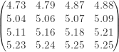
San Francisco rainfall data
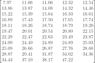
The following table shows the annual rainfall data in San Francisco (in inches) from 1960-2013 (data source). The table consits of 54 measurements and is sorted in increasing order from left to right (and from top to bottom). Each annual rainfall measurement is from July of that year to June of the following year. The driest year (7.97 inches) is 1975, the period from July 1975 to June 1976. The wettest year (47.22 inches) is 1997, which is the period from July 1997 to June 1998. The most recent data point is the fifth measurement 12.54 inches (the period from July 2013 to June 2014).
Using the above data, estimate the median, the lower quartile (25th percentile) and the upper quartile (the 75th percentile) of the annual rainfall in San Francisco. Then find a reasonably good confidence interval for each of the three population percentiles.
________________________________________________________________________
Basic facts about order statistics
Let’s recall some basic facts from the following previous posts:
Let’s say we have a random sample  drawn from a population whose percentiles are unknown and we wish to estimate them. Rank the items of the random sample to obtain the order statistics
  . In an ideal setting, the measurements are supposed to arise from a continuous distribution. So the chance of a tie among the
  is zero. But this assumption may not hold on occasions. There are some ties in the San Francisco rainfall data (e.g. the second and third data point). The small number of ties will not affect the calculation performed below.
The reason that we can use the order statistics to estimate the population percentiles is that the expected percentage of the population below is about the same as the percentage of the sample items less than . According to the explanation in the second post listed above (link), the order statistic is expected to be above  percent of the population where
  . In fact, the order statistics are expected to divide the population in roughly equal segments. More specifically the expected percentage of the population in between
  and is
  where
where  .
.
The above explanation justifies the use of the order statistic as the sample th percentile where .
The sample size is  54 in the San Francisco rainfall data. Thus the order statistic
  is the sample 20th percentile and can be taken as an estimate of the population 20th percentile for the San Francisco annual rainfall. Here the realized value of is 15.22.
With  , the order statistic
  is the sample 82nd percentile and is taken as an estimate of the population 82nd percentile for the San Francisco annual rainfall. The realized value of is 28.68 inches.
The key for constructing confidence interval for percentiles is to calculate the probability  . This is the probability that the th percentile, where
  , is in between
  and . Let's look at the median
  . For
. For  to happen, there must be at least
  many sample items less than the median . For
  to happen, there can be at most
  many sample items less than the median . Thus in the random draws of the sample items, in order for the event
  to occur, there must be at least sample items and at most sample items that are less than . In other words, in
  Bernoulli trials, there at at least and at most successes where the probability of success is
  0.5. The following is the probability
  :
:
Then interval is taken to be the  % confidence interval for the unknown population median . Note that this confidence interval is constructed without knowing (or assuming) anything about the underlying distribution of the population.
Consider the th percentile where . In order for the event  to occur, there must be at least sample items and at most sample items that are less than
  . This is equivalent to Bernoulli trials resulting in at least successes and at most successes where the probability of success is
  .
.
Then interval is taken to be the % confidence interval for the unknown population percentile . As mentioned earlier, this confidence interval does not need to rely on any information about the distribution of the population and is said to be distribution free. It only relies on a probability statement that involves the binomial distribution in describing the positioning of the sample items. In the past, people used normal approximation to the binomial to estimate this probability. The normal approximation should be no longer needed as computing software is now easily available. For example, binomial probabilities can be computed in Excel for number of trials a million or more.
________________________________________________________________________
Percentiles of annual rainfall
Using the above data, estimate the median, the lower quartile (25th percentile) and the upper quartile (the 75th percentile) of the annual rainfall in San Francisco. Then find a reasonably good confidence interval for each of the three population percentiles.
The sample size is 54. The middle two data elements in the sample is  and
and  . They are realizations of the order statistics
  and
and  . So in this example,
  and
and  . Thus the order statistic is expected to be greater than about 49% of the population and is expected to be greater than about 51% of the population. So neither nor is an exact fit. So we take the average of the two as an estimate of the population median:
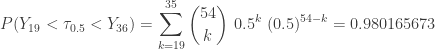
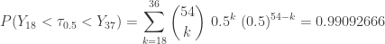
Looking for confidence intervals, we consider the intervals  ,
,  ,
,  and
and  . The following shows the confidence levels.
The above calculation is done in Excel. The binomial probabilities are done using the function BINOM.DIST. So we have the following confidence intervals for the median annual San Francisco rainfall in inches.
Median

= (18.11, 23.49) with approximately 92% confidence
= (17.74, 23.87) with approximately 96% confidence
= (17.65, 24.09) with approximately 98% confidence
= (17.50, 24.49) with approximately 99% confidence
For the lower quartile and upper quartile, the following are the results. The reader is invited to confirm the calculation.
Lower quartile
 , average of
  and
and 
 = (13.87, 17.74) with approximately 96% confidence
 = (13.86, 18.11) with approximately 98% confidence
 = (12.54, 18.26) with approximately 99% confidence
Upper quartile
 , average of
  and
and 
 = (24.09, 29.41) with approximately 91% confidence
 = (23.87, 31.87) with approximately 96% confidence
 = (23.49, 34.02) with approximately 98% confidence
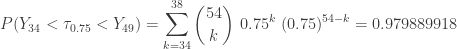
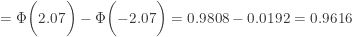
The following shows the calculation for two of the confidence intervals, one for  and one for
  .
.
________________________________________________________________________


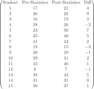
 be the post-statistics score on the diagnostic test and let
  be the pre-statistics score on the disgnostic test. Let
 ![p=P[X>Y]](https://s0.wp.com/latex.php?latex=p%3DP%5BX%3EY%5D&bg=ffffff&fg=333333&s=-1&c=20201002) . This is the probability that the student has an improvement on the quantitative test after taking a one-semester introductory statistics course. The test hypotheses are as follows:
. This is the probability that the student has an improvement on the quantitative test after taking a one-semester introductory statistics course. The test hypotheses are as follows:
 be the number of students with an improvement between the post and pre scores. Since there are two students with a zero difference, under
  ,
,  . Then the observed value of
  . The following is the P-value:
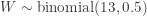
![\displaystyle \text{P-value}=P[W \ge 9]=\sum \limits_{k=9}^{13} \binom{13}{k} \biggl(\frac{1}{2}\biggr)^{13}=0.1334](https://s0.wp.com/latex.php?latex=%5Cdisplaystyle+%5Ctext%7BP-value%7D%3DP%5BW+%5Cge+9%5D%3D%5Csum+%5Climits_%7Bk%3D9%7D%5E%7B13%7D+%5Cbinom%7B13%7D%7Bk%7D+%5Cbiggl%28%5Cfrac%7B1%7D%7B2%7D%5Cbiggr%29%5E%7B13%7D%3D0.1334&bg=ffffff&fg=333333&s=-1&c=20201002)
 being the mean of
  , the hypotheses for the t-test are:
 be the pH level of a sample of rainwater in this region of Washington state. Let
 ![p=P[5.2>X]=P[5.2-X>0]](https://s0.wp.com/latex.php?latex=p%3DP%5B5.2%3EX%5D%3DP%5B5.2-X%3E0%5D&bg=ffffff&fg=333333&s=-1&c=20201002) . Thus
. Thus  is the probability of a plus sign when comparing the each data measurement and 5.2. The hypotheses to be tested are:
 ). Then
 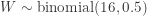 . There are 11 data measurements with plus signs (
 ). Thus the P-value is:
![\displaystyle \text{P-value}=P[W \ge 11]=\sum \limits_{k=11}^{16} \binom{16}{k} \biggl(\frac{1}{2}\biggr)^{16}=0.1051](https://s0.wp.com/latex.php?latex=%5Cdisplaystyle+%5Ctext%7BP-value%7D%3DP%5BW+%5Cge+11%5D%3D%5Csum+%5Climits_%7Bk%3D11%7D%5E%7B16%7D+%5Cbinom%7B16%7D%7Bk%7D+%5Cbiggl%28%5Cfrac%7B1%7D%7B2%7D%5Cbiggr%29%5E%7B16%7D%3D0.1051&bg=ffffff&fg=333333&s=-1&c=20201002)
 , the null hypothesis is not rejected. We still believe that the rainwater in this region is not acidic.
 of the students in the sample prefer instructor B over A. This seems like convincing evidence that B is indeed more popular. Let perform some calculation to confirm this. Let
 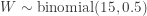 . Then the P-value is:
![\displaystyle \text{P-value}=P[W \ge 11]=\sum \limits_{k=11}^{15} \binom{15}{k} \biggl(\frac{1}{2}\biggr)^{15}=0.05923](https://s0.wp.com/latex.php?latex=%5Cdisplaystyle+%5Ctext%7BP-value%7D%3DP%5BW+%5Cge+11%5D%3D%5Csum+%5Climits_%7Bk%3D11%7D%5E%7B15%7D+%5Cbinom%7B15%7D%7Bk%7D+%5Cbiggl%28%5Cfrac%7B1%7D%7B2%7D%5Cbiggr%29%5E%7B15%7D%3D0.05923&bg=ffffff&fg=333333&s=-1&c=20201002)
 is close to normal and the t-procedure is robust. If the sample size is small and the underlying distribution is clearly not normal (e.g. is extremely skewed), what significance test do we use? Let’s take the example of a matched pairs data problem. The matched pairs t-test is to test the hypothesis that there is “no difference” between two continuous random variables
  is a pair of continuous random variables. Suppose that a random sample of paired data
  is obtained. We omit the observations
  with
with  . Let
. Let  be the number of pairs for which
  . For each of these
  (
( if
if  and
and  if
if  ). Let
  , then any random pair
  is the hypothesis of “no difference”. Under this hypothesis, there is no difference between the two measurements

 . When
  . Thus the binomial distribution is used for calculating significance. The left-tailed P-value is of the form
 ![P[W \le w]](https://s0.wp.com/latex.php?latex=P%5BW+%5Cle+w%5D&bg=ffffff&fg=333333&s=-1&c=20201002) and the right-tailed P-value is
and the right-tailed P-value is ![P[W \ge w]](https://s0.wp.com/latex.php?latex=P%5BW+%5Cge+w%5D&bg=ffffff&fg=333333&s=-1&c=20201002) . Then the two-tailed P-value is twice the one-sided P-value.
. Then the two-tailed P-value is twice the one-sided P-value. be the median of the differences
  . For the alternative hypotheses, we have the following equivalences:


![\displaystyle H_0:p=\frac{1}{2} \ \ \ \ \ H_1:p>\frac{1}{2} \ \ \ \text{where} \ p=P[X>Y]](https://s0.wp.com/latex.php?latex=%5Cdisplaystyle+H_0%3Ap%3D%5Cfrac%7B1%7D%7B2%7D+%5C+%5C+%5C+%5C+%5C+H_1%3Ap%3E%5Cfrac%7B1%7D%7B2%7D+%5C+%5C+%5C+%5Ctext%7Bwhere%7D+%5C+p%3DP%5BX%3EY%5D&bg=ffffff&fg=333333&s=-1&c=20201002)
 . Then
  . The observed value of the statistic
  . Since this is a right-tailed test, the following is the P-value:
![\displaystyle \text{P-value}=P[W \ge 15]=\sum \limits_{k=15}^{20} \binom{20}{k} \biggl(\frac{1}{2}\biggr)^{20}=0.02069](https://s0.wp.com/latex.php?latex=%5Cdisplaystyle+%5Ctext%7BP-value%7D%3DP%5BW+%5Cge+15%5D%3D%5Csum+%5Climits_%7Bk%3D15%7D%5E%7B20%7D+%5Cbinom%7B20%7D%7Bk%7D+%5Cbiggl%28%5Cfrac%7B1%7D%7B2%7D%5Cbiggr%29%5E%7B20%7D%3D0.02069&bg=ffffff&fg=333333&s=-1&c=20201002)


 . The observed value of the statistic
  . Since this is a right-tailed test, the following is the P-value:
![\displaystyle \text{P-value}=P[W \ge 12]=\sum \limits_{k=12}^{17} \binom{17}{k} \biggl(\frac{1}{2}\biggr)^{17}=0.07173](https://s0.wp.com/latex.php?latex=%5Cdisplaystyle+%5Ctext%7BP-value%7D%3DP%5BW+%5Cge+12%5D%3D%5Csum+%5Climits_%7Bk%3D12%7D%5E%7B17%7D+%5Cbinom%7B17%7D%7Bk%7D+%5Cbiggl%28%5Cfrac%7B1%7D%7B2%7D%5Cbiggr%29%5E%7B17%7D%3D0.07173&bg=ffffff&fg=333333&s=-1&c=20201002)
 , we reject the null hypothesis. However, we would like to add a caveat. The value of this example is that it is an excellent demonstration of the sign test. The 17 oil changes are not controlled. For example, the data are just records of mileage and gas usage for 17 oil changes (both pre and post). No effort was made to make sure that the driving conditions are similar for the pre oil change MPG and post oil change MPG (freeway vs. local streets, weather conditions, etc). With more care in producing the data, we can conceivably derive a more definite answer.
 , the
, the  order statistic
  is the sample
  percentile and is an estimate of the unknown population
  . The justification is that the area under the density curve of the distribution and to the left of
  (see the discussion below). The order statistics can also be used for constructing confidence intervals for unknown population percentiles. Such confidence intervals are often called distribution-free confidence intervals because no information about the underlying distribution is used in the construction. In the previous post (
 be a random sample drawn from a continuous distribution with
  and
and  denoting the common random variable, the common distribution function and probability density function, respectively. Let
  be the associated order statistics. Let
  . Note that
  can be interpreted as an area under the density curve:
![\displaystyle E[W_i]=\frac{i}{n+1}](https://s0.wp.com/latex.php?latex=%5Cdisplaystyle+E%5BW_i%5D%3D%5Cfrac%7Bi%7D%7Bn%2B1%7D&bg=ffffff&fg=333333&s=-1&c=20201002) . On this basis,
. On this basis,  is defined as the sample
  percentile where
  and is used as an estimate for the unknown population
 ![P[Y_i < \tau_p < Y_j]](https://s0.wp.com/latex.php?latex=P%5BY_i+%3C+%5Ctau_p+%3C+Y_j%5D&bg=ffffff&fg=333333&s=-1&c=20201002) where
where  is the
 ![P[Y_2 < \tau_{0.5} < Y_8]](https://s0.wp.com/latex.php?latex=P%5BY_2+%3C+%5Ctau_%7B0.5%7D+%3C+Y_8%5D&bg=ffffff&fg=333333&s=-1&c=20201002) . For
. For  to happen, there must be at least two sample items
  that are less than
  . For
. For  to happen, there can be no more than 8 sample items
  as a success. The probability of a success is thus
 ![p=P[X<\tau_{0.5}]=0.5](https://s0.wp.com/latex.php?latex=p%3DP%5BX%3C%5Ctau_%7B0.5%7D%5D%3D0.5&bg=ffffff&fg=333333&s=-1&c=20201002) . We are interested in the probability of having at least 2 and at most 7 successes. Thus we have:
. We are interested in the probability of having at least 2 and at most 7 successes. Thus we have:![\displaystyle P[Y_2 < \tau_{0.5} < Y_8]=\sum \limits_{k=2}^{7} \binom{n}{k} \biggl(\frac{1}{2}\biggr)^k \biggl(\frac{1}{2}\biggr)^{n-k}=1-\alpha](https://s0.wp.com/latex.php?latex=%5Cdisplaystyle+P%5BY_2+%3C+%5Ctau_%7B0.5%7D+%3C+Y_8%5D%3D%5Csum+%5Climits_%7Bk%3D2%7D%5E%7B7%7D+%5Cbinom%7Bn%7D%7Bk%7D+%5Cbiggl%28%5Cfrac%7B1%7D%7B2%7D%5Cbiggr%29%5Ek+%5Cbiggl%28%5Cfrac%7B1%7D%7B2%7D%5Cbiggr%29%5E%7Bn-k%7D%3D1-%5Calpha&bg=ffffff&fg=333333&s=-1&c=20201002)
 is taken to be the
  % confidence interval for the unknown population median.
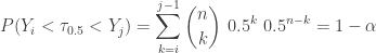
![p=P[X < \tau_p]](https://s0.wp.com/latex.php?latex=p%3DP%5BX+%3C+%5Ctau_p%5D&bg=ffffff&fg=333333&s=-1&c=20201002) .
.![\displaystyle P[Y_i < \tau_{p} < Y_j]=\sum \limits_{k=i}^{j-1} \binom{n}{k} p^k (1-p)^{n-k}=1-\alpha](https://s0.wp.com/latex.php?latex=%5Cdisplaystyle+P%5BY_i+%3C+%5Ctau_%7Bp%7D+%3C+Y_j%5D%3D%5Csum+%5Climits_%7Bk%3Di%7D%5E%7Bj-1%7D+%5Cbinom%7Bn%7D%7Bk%7D+p%5Ek+%281-p%29%5E%7Bn-k%7D%3D1-%5Calpha&bg=ffffff&fg=333333&s=-1&c=20201002)
 is taken to be the
  . Its mean is
  and its variance is
  . This fact becomes useful when using normal approximation of the above probability.
 has a higher confidence level than the inteval
  . Note that of the two probabilities below, the first one is higher.
![\displaystyle P[Y_2 < \tau_{0.5} < Y_{15}]=\sum \limits_{k=2}^{14} \binom{n}{k} \biggl(\frac{1}{2}\biggr)^k \biggl(\frac{1}{2}\biggr)^{n-k}](https://s0.wp.com/latex.php?latex=%5Cdisplaystyle+P%5BY_2+%3C+%5Ctau_%7B0.5%7D+%3C+Y_%7B15%7D%5D%3D%5Csum+%5Climits_%7Bk%3D2%7D%5E%7B14%7D+%5Cbinom%7Bn%7D%7Bk%7D+%5Cbiggl%28%5Cfrac%7B1%7D%7B2%7D%5Cbiggr%29%5Ek+%5Cbiggl%28%5Cfrac%7B1%7D%7B2%7D%5Cbiggr%29%5E%7Bn-k%7D&bg=ffffff&fg=333333&s=-1&c=20201002)
![\displaystyle P[Y_6 < \tau_{0.5} < Y_{10}]=\sum \limits_{k=6}^{9} \binom{n}{k} \biggl(\frac{1}{2}\biggr)^k \biggl(\frac{1}{2}\biggr)^{n-k}](https://s0.wp.com/latex.php?latex=%5Cdisplaystyle+P%5BY_6+%3C+%5Ctau_%7B0.5%7D+%3C+Y_%7B10%7D%5D%3D%5Csum+%5Climits_%7Bk%3D6%7D%5E%7B9%7D+%5Cbinom%7Bn%7D%7Bk%7D+%5Cbiggl%28%5Cfrac%7B1%7D%7B2%7D%5Cbiggr%29%5Ek+%5Cbiggl%28%5Cfrac%7B1%7D%7B2%7D%5Cbiggr%29%5E%7Bn-k%7D&bg=ffffff&fg=333333&s=-1&c=20201002)
 grocery purchased amounts of a certain family in 2009. The data are arranged in increasing order on each row from left to right.
 , the
, the  grocery purchase. The upper quartile (
 percentile) is the
  grocery purchase 101.81.
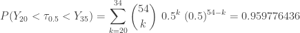
![P[Y_i< \tau_{0.5} < Y_j]](https://s0.wp.com/latex.php?latex=P%5BY_i%3C+%5Ctau_%7B0.5%7D+%3C+Y_j%5D&bg=ffffff&fg=333333&s=-1&c=20201002) . We use the interval
. We use the interval  because of the following probability:
![\displaystyle P[Y_{4} < \tau_{0.5} < Y_{12}]=\sum \limits_{k=4}^{11} \binom{15}{k} \biggl(\frac{1}{2}\biggr)^k \biggl(\frac{1}{2}\biggr)^{n-k}=0.96484375](https://s0.wp.com/latex.php?latex=%5Cdisplaystyle+P%5BY_%7B4%7D+%3C+%5Ctau_%7B0.5%7D+%3C+Y_%7B12%7D%5D%3D%5Csum+%5Climits_%7Bk%3D4%7D%5E%7B11%7D+%5Cbinom%7B15%7D%7Bk%7D+%5Cbiggl%28%5Cfrac%7B1%7D%7B2%7D%5Cbiggr%29%5Ek+%5Cbiggl%28%5Cfrac%7B1%7D%7B2%7D%5Cbiggr%29%5E%7Bn-k%7D%3D0.96484375&bg=ffffff&fg=333333&s=-1&c=20201002)
 is an approximate 96% confidence interval for the median grocery purchase amount for this family. The above calculation is made using an Excel spread sheet. Let's compare this answer with a normal approximation. The mean of the binomial distribution in question is
  and the variance is
  . Consider the following:
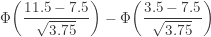

 and common density function
  . The order statistics
  is the smallest item in the sample and
  is the second smallest item in the sample and so on. Since this is random sampling from a continuous distribution, we assume that the probability of a tie between two order statistics is zero. In the previous post
  order statistic:
![\displaystyle f_{Y_i}(y)=\frac{n!}{(i-1)! (n-i)!} \thinspace F(y)^{i-1} \thinspace [1-F(y)]^{n-i} f(y)](https://s0.wp.com/latex.php?latex=%5Cdisplaystyle+f_%7BY_i%7D%28y%29%3D%5Cfrac%7Bn%21%7D%7B%28i-1%29%21+%28n-i%29%21%7D+%5Cthinspace+F%28y%29%5E%7Bi-1%7D+%5Cthinspace+%5B1-F%28y%29%5D%5E%7Bn-i%7D+f%28y%29&bg=ffffff&fg=333333&s=-1&c=20201002)
 . Since the distribution function of
  where
where  , the probability density function of the
 ![\displaystyle f_{Y_i}(y)=\frac{n!}{(i-1)! (n-i)!} \thinspace y^{i-1} \thinspace [1-y]^{n-i}](https://s0.wp.com/latex.php?latex=%5Cdisplaystyle+f_%7BY_i%7D%28y%29%3D%5Cfrac%7Bn%21%7D%7B%28i-1%29%21+%28n-i%29%21%7D+%5Cthinspace+y%5E%7Bi-1%7D+%5Cthinspace+%5B1-y%5D%5E%7Bn-i%7D&bg=ffffff&fg=333333&s=-1&c=20201002) where
where ![\displaystyle f_{W}(w)=\frac{\Gamma(a+b)}{\Gamma(a) \Gamma(b)} \thinspace w^{a-1} \thinspace [1-w]^{b-1}](https://s0.wp.com/latex.php?latex=%5Cdisplaystyle+f_%7BW%7D%28w%29%3D%5Cfrac%7B%5CGamma%28a%2Bb%29%7D%7B%5CGamma%28a%29+%5CGamma%28b%29%7D+%5Cthinspace+w%5E%7Ba-1%7D+%5Cthinspace+%5B1-w%5D%5E%7Bb-1%7D&bg=ffffff&fg=333333&s=-1&c=20201002) where
where  where
where  is the gamma function.
![\displaystyle E[W]=\frac{a}{a+b}](https://s0.wp.com/latex.php?latex=%5Cdisplaystyle+E%5BW%5D%3D%5Cfrac%7Ba%7D%7Ba%2Bb%7D&bg=ffffff&fg=333333&s=-1&c=20201002)
![\displaystyle Var[W]=\frac{ab}{(a+b)^2 (a+b+1)}](https://s0.wp.com/latex.php?latex=%5Cdisplaystyle+Var%5BW%5D%3D%5Cfrac%7Bab%7D%7B%28a%2Bb%29%5E2+%28a%2Bb%2B1%29%7D&bg=ffffff&fg=333333&s=-1&c=20201002)
![\displaystyle f_{Y_i}(y)=\frac{\Gamma(n+1)}{\Gamma(i) \Gamma(n-i+1)} \thinspace y^{i-1} \thinspace [1-y]^{(n-i+1)-1}](https://s0.wp.com/latex.php?latex=%5Cdisplaystyle+f_%7BY_i%7D%28y%29%3D%5Cfrac%7B%5CGamma%28n%2B1%29%7D%7B%5CGamma%28i%29+%5CGamma%28n-i%2B1%29%7D+%5Cthinspace+y%5E%7Bi-1%7D+%5Cthinspace+%5B1-y%5D%5E%7B%28n-i%2B1%29-1%7D&bg=ffffff&fg=333333&s=-1&c=20201002) where
where ![\displaystyle E[Y_i]=\frac{i}{i+(n-i+1)}=\frac{i}{n+1}](https://s0.wp.com/latex.php?latex=%5Cdisplaystyle+E%5BY_i%5D%3D%5Cfrac%7Bi%7D%7Bi%2B%28n-i%2B1%29%7D%3D%5Cfrac%7Bi%7D%7Bn%2B1%7D&bg=ffffff&fg=333333&s=-1&c=20201002)
![\displaystyle Var[Y_i]=\frac{i(n-i+1)}{(n+1)^2 (n+2)}](https://s0.wp.com/latex.php?latex=%5Cdisplaystyle+Var%5BY_i%5D%3D%5Cfrac%7Bi%28n-i%2B1%29%7D%7B%28n%2B1%29%5E2+%28n%2B2%29%7D&bg=ffffff&fg=333333&s=-1&c=20201002)
 , then the sample median is the order statistic
  . The preceding discussion on the order statistics of the uniform distribution can show us that this approach is a sound one.
 , consider
  are also increasing:
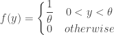
 follows the uniform distribution
 are the order statistics for this random sample. By the preceding discussion,
 ![\displaystyle E[W_i]=E[F(Y_i)]=\frac{i}{n+1}](https://s0.wp.com/latex.php?latex=%5Cdisplaystyle+E%5BW_i%5D%3DE%5BF%28Y_i%29%5D%3D%5Cfrac%7Bi%7D%7Bn%2B1%7D&bg=ffffff&fg=333333&s=-1&c=20201002) . Note that
. Note that ![E[W_i]=E[F(Y_i)]](https://s0.wp.com/latex.php?latex=E%5BW_i%5D%3DE%5BF%28Y_i%29%5D&bg=ffffff&fg=333333&s=-1&c=20201002) is the expected area under the density curve
is the expected area under the density curve  is the common density function of the original sample
  . Then the sample median is
 ![\displaystyle E[W_{m+1}]=\frac{m+1}{n+1}=\frac{1}{2}](https://s0.wp.com/latex.php?latex=%5Cdisplaystyle+E%5BW_%7Bm%2B1%7D%5D%3D%5Cfrac%7Bm%2B1%7D%7Bn%2B1%7D%3D%5Cfrac%7B1%7D%7B2%7D&bg=ffffff&fg=333333&s=-1&c=20201002) . Thus if we choose
. Thus if we choose ![E[W_i - W_{i-1}]](https://s0.wp.com/latex.php?latex=E%5BW_i+-+W_%7Bi-1%7D%5D&bg=ffffff&fg=333333&s=-1&c=20201002) is the expected area under the density curve and between
is the expected area under the density curve and between  . This expected area is:
![\displaystyle E[W_i - W_{i-1}]=E[F(Y_i)]-E[F(Y_{i-1})]=\frac{i}{n+1}-\frac{i-1}{n+1}=\frac{1}{n+1}](https://s0.wp.com/latex.php?latex=%5Cdisplaystyle+E%5BW_i+-+W_%7Bi-1%7D%5D%3DE%5BF%28Y_i%29%5D-E%5BF%28Y_%7Bi-1%7D%29%5D%3D%5Cfrac%7Bi%7D%7Bn%2B1%7D-%5Cfrac%7Bi-1%7D%7Bn%2B1%7D%3D%5Cfrac%7B1%7D%7Bn%2B1%7D&bg=ffffff&fg=333333&s=-1&c=20201002)
 is:
is:![\displaystyle E[1-F(Y_n)]=1-\frac{n}{n+1}=\frac{1}{n+1}](https://s0.wp.com/latex.php?latex=%5Cdisplaystyle+E%5B1-F%28Y_n%29%5D%3D1-%5Cfrac%7Bn%7D%7Bn%2B1%7D%3D%5Cfrac%7B1%7D%7Bn%2B1%7D&bg=ffffff&fg=333333&s=-1&c=20201002)
 . The order statistics
  areas. On average each of these area is
  .
. where the area under the density curve
  is not an integer, then we interpolate between two order statistics. For example, if
  , then we interpolate between
  and
and  drawn from a continuous distribution. Find estimators for the median, first quartile and second quartile. Find an estimate for the
  percentile. Construct an 87% confidence interval for the
  percentile.
 percentile) is third order statistic
  . The estimator for the second quartile (
 . Based on the preceding discussion, the expected area under the density curve
  are 0.25, 0.5 and 0.75, respectively.
 . Thus we interpolate
  and
and  . In our example, we use linear interpolation, though taking the arithmetic average of
![P[Y_2 < \tau_{0.4} < Y_7]](https://s0.wp.com/latex.php?latex=P%5BY_2+%3C+%5Ctau_%7B0.4%7D+%3C+Y_7%5D&bg=ffffff&fg=333333&s=-1&c=20201002) where
where  is the
  percentile. Consider the event
  as a success with probability of success
  . For
. For  to happen, there must be at least 2 successes and fewer than 7 success in the binomial distribution with
  . Thus we have:
![\displaystyle P[Y_2 < \tau_{0.4} < Y_7]=\sum \limits_{j=2}^{6} \binom{11}{j} 0.4^{j} 0.6^{11-j}=0.8704](https://s0.wp.com/latex.php?latex=%5Cdisplaystyle+P%5BY_2+%3C+%5Ctau_%7B0.4%7D+%3C+Y_7%5D%3D%5Csum+%5Climits_%7Bj%3D2%7D%5E%7B6%7D+%5Cbinom%7B11%7D%7Bj%7D+0.4%5E%7Bj%7D+0.6%5E%7B11-j%7D%3D0.8704&bg=ffffff&fg=333333&s=-1&c=20201002)
 can be taken as the 87% confidence interval for
  . This is an example of a distribution-free confidence interval because nothing is assumed about the underlying distribution in the construction of the confidence interval.
 . In other words, we have:
 the smallest of
  the second smallest of
 the largest of
  and
and  . The order statistic
  occurs, then there are at least
  in the sample that are less than or equal to
  . Consider the event that
  as a success and
 ![F(y)=P[X \le y]](https://s0.wp.com/latex.php?latex=F%28y%29%3DP%5BX+%5Cle+y%5D&bg=ffffff&fg=333333&s=-1&c=20201002) as the probability of success. Then the drawing of each sample item becomes a Bernoulli trial (a success or a failure). We are interested in the probability of having at least
as the probability of success. Then the drawing of each sample item becomes a Bernoulli trial (a success or a failure). We are interested in the probability of having at least ![\displaystyle F_{Y_i}(y)=P[Y_i \le y]=\sum \limits_{k=i}^{n} \binom{n}{k} F(y)^k [1-F(y)]^{n-k}\ \ \ \ \ \ \ \ \ \ \ \ (1)](https://s0.wp.com/latex.php?latex=%5Cdisplaystyle+F_%7BY_i%7D%28y%29%3DP%5BY_i+%5Cle+y%5D%3D%5Csum+%5Climits_%7Bk%3Di%7D%5E%7Bn%7D+%5Cbinom%7Bn%7D%7Bk%7D+F%28y%29%5Ek+%5B1-F%28y%29%5D%5E%7Bn-k%7D%5C+%5C+%5C+%5C+%5C+%5C+%5C+%5C+%5C+%5C+%5C+%5C++%281%29&bg=ffffff&fg=333333&s=0&c=20201002)
![\displaystyle F_{Y_i}(y)=F_{Y_{i-1}}(y)-\binom{n}{i-1} F(y)^{i-1} [1-F(y)]^{n-i+1} \ \ \ \ \ \ \ \ \ \ \ \ \ \ \ (2)](https://s0.wp.com/latex.php?latex=%5Cdisplaystyle+F_%7BY_i%7D%28y%29%3DF_%7BY_%7Bi-1%7D%7D%28y%29-%5Cbinom%7Bn%7D%7Bi-1%7D+F%28y%29%5E%7Bi-1%7D+%5B1-F%28y%29%5D%5E%7Bn-i%2B1%7D+%5C+%5C+%5C+%5C+%5C+%5C+%5C+%5C+%5C+%5C+%5C+%5C+%5C+%5C+%5C+%282%29&bg=ffffff&fg=333333&s=-1&c=20201002)
![\displaystyle f_{Y_i}(y)=\frac{n!}{(i-1)! (n-i)!} \thinspace F(y)^{i-1} \thinspace [1-F(y)]^{n-i} f_X(y) \ \ \ \ \ \ \ \ \ \ \ \ \ \ \ (3)](https://s0.wp.com/latex.php?latex=%5Cdisplaystyle+f_%7BY_i%7D%28y%29%3D%5Cfrac%7Bn%21%7D%7B%28i-1%29%21+%28n-i%29%21%7D+%5Cthinspace+F%28y%29%5E%7Bi-1%7D+%5Cthinspace+%5B1-F%28y%29%5D%5E%7Bn-i%7D+f_X%28y%29+%5C+%5C+%5C+%5C+%5C+%5C+%5C+%5C+%5C+%5C+%5C+%5C+%5C+%5C+%5C+%283%29&bg=ffffff&fg=333333&s=-1&c=20201002)
 . Note that
  is the probability that at least one
  and is the complement of the probability of having no
 ![F_{Y_1}(y)=1-[1-F(y)]^n](https://s0.wp.com/latex.php?latex=F_%7BY_1%7D%28y%29%3D1-%5B1-F%28y%29%5D%5En&bg=ffffff&fg=333333&s=-1&c=20201002) . By taking derivative, we have:
. By taking derivative, we have:![\displaystyle f_{Y_1}(y)=F_{Y_1}^{-1}(y)=n [1-F(y)]^{n-1} f_X(y)](https://s0.wp.com/latex.php?latex=%5Cdisplaystyle+f_%7BY_1%7D%28y%29%3DF_%7BY_1%7D%5E%7B-1%7D%28y%29%3Dn+%5B1-F%28y%29%5D%5E%7Bn-1%7D+f_X%28y%29&bg=ffffff&fg=333333&s=-1&c=20201002)
![\displaystyle f_{Y_{i-1}}(y)=\frac{n!}{(i-2)! (n-i+1)!} \thinspace F(y)^{i-2} \thinspace [1-F(y)]^{n-i+1} f_X(y)](https://s0.wp.com/latex.php?latex=%5Cdisplaystyle+f_%7BY_%7Bi-1%7D%7D%28y%29%3D%5Cfrac%7Bn%21%7D%7B%28i-2%29%21+%28n-i%2B1%29%21%7D+%5Cthinspace+F%28y%29%5E%7Bi-2%7D+%5Cthinspace+%5B1-F%28y%29%5D%5E%7Bn-i%2B1%7D+f_X%28y%29&bg=ffffff&fg=333333&s=-1&c=20201002)
![\displaystyle f_{Y_i}(y)=f_{Y_{i-1}}(y)-\biggl[(i-1)\binom{n}{i-1} F(y)^{i-2} f_X(y)[1-F(y)]^{n-i+1}](https://s0.wp.com/latex.php?latex=%5Cdisplaystyle+f_%7BY_i%7D%28y%29%3Df_%7BY_%7Bi-1%7D%7D%28y%29-%5Cbiggl%5B%28i-1%29%5Cbinom%7Bn%7D%7Bi-1%7D+F%28y%29%5E%7Bi-2%7D+f_X%28y%29%5B1-F%28y%29%5D%5E%7Bn-i%2B1%7D&bg=ffffff&fg=333333&s=-1&c=20201002)
![\displaystyle -\ \ \ \ \ \ \ \ \ \ \binom{n}{i-1}F(y)^{i-1}(n-i+1)[1-F(y)]^{n-i} f_X(y) \biggr]](https://s0.wp.com/latex.php?latex=%5Cdisplaystyle+-%5C+%5C+%5C+%5C+%5C+%5C+%5C+%5C+%5C+%5C+%5Cbinom%7Bn%7D%7Bi-1%7DF%28y%29%5E%7Bi-1%7D%28n-i%2B1%29%5B1-F%28y%29%5D%5E%7Bn-i%7D+f_X%28y%29+%5Cbiggr%5D&bg=ffffff&fg=333333&s=-1&c=20201002)
![\displaystyle F(y)^{i-1} \thinspace f_X(y) \thinspace [1-F(y)]^{n-i}](https://s0.wp.com/latex.php?latex=%5Cdisplaystyle+F%28y%29%5E%7Bi-1%7D+%5Cthinspace+f_X%28y%29+%5Cthinspace+%5B1-F%28y%29%5D%5E%7Bn-i%7D&bg=ffffff&fg=333333&s=-1&c=20201002)
 sample items below
  items above
 ![\displaystyle f_{Y_i}(y)=\frac{n!}{(i-1)! 1! (n-i)!} \thinspace F(y)^{i-1} \thinspace f_X(y) \thinspace [1-F(y)]^{n-i} \ \ \ \ \ \ \ \ \ \ \ \ \ \ \ (4)](https://s0.wp.com/latex.php?latex=%5Cdisplaystyle+f_%7BY_i%7D%28y%29%3D%5Cfrac%7Bn%21%7D%7B%28i-1%29%21+1%21+%28n-i%29%21%7D+%5Cthinspace+F%28y%29%5E%7Bi-1%7D+%5Cthinspace+f_X%28y%29+%5Cthinspace+%5B1-F%28y%29%5D%5E%7Bn-i%7D+%5C+%5C+%5C+%5C+%5C+%5C+%5C+%5C+%5C+%5C+%5C+%5C+%5C+%5C+%5C+%284%29&bg=ffffff&fg=333333&s=-1&c=20201002)
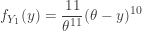
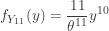
 . Find the pdfs for
  and
and ![E[Y_6]](https://s0.wp.com/latex.php?latex=E%5BY_6%5D&bg=ffffff&fg=333333&s=-1&c=20201002) .
. . The distribution function and pdf of
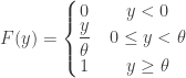
 . As an estimator of the median, we prefer
 ![E[Y_6]=\frac{\theta}{2}](https://s0.wp.com/latex.php?latex=E%5BY_6%5D%3D%5Cfrac%7B%5Ctheta%7D%7B2%7D&bg=ffffff&fg=333333&s=-1&c=20201002) .
.![\displaystyle E[Y_6]=\int_0^{\theta}2772 y \biggl(\frac{y}{\theta}\biggr)^5 \biggl(1-\frac{y}{\theta}\biggr)^5 \frac{1}{\theta} dy](https://s0.wp.com/latex.php?latex=%5Cdisplaystyle+E%5BY_6%5D%3D%5Cint_0%5E%7B%5Ctheta%7D2772+y+%5Cbiggl%28%5Cfrac%7By%7D%7B%5Ctheta%7D%5Cbiggr%29%5E5+%5Cbiggl%281-%5Cfrac%7By%7D%7B%5Ctheta%7D%5Cbiggr%29%5E5+%5Cfrac%7B1%7D%7B%5Ctheta%7D+dy&bg=ffffff&fg=333333&s=-1&c=20201002)
 , we have the following beta integral.
![\displaystyle E[Y_6]=2772 \theta \int_0^1 w^{7-1} (1-w)^{6-1} dw](https://s0.wp.com/latex.php?latex=%5Cdisplaystyle+E%5BY_6%5D%3D2772+%5Ctheta+%5Cint_0%5E1+w%5E%7B7-1%7D+%281-w%29%5E%7B6-1%7D+dw&bg=ffffff&fg=333333&s=-1&c=20201002)
![\displaystyle E[Y_6]=2772 \theta \thinspace \frac{\Gamma(7) \Gamma(6)}{\Gamma(13)}=2772 \theta \thinspace \frac{6! \thinspace 5!}{12!}=\frac{\theta}{2}](https://s0.wp.com/latex.php?latex=%5Cdisplaystyle+E%5BY_6%5D%3D2772+%5Ctheta+%5Cthinspace+%5Cfrac%7B%5CGamma%287%29+%5CGamma%286%29%7D%7B%5CGamma%2813%29%7D%3D2772+%5Ctheta+%5Cthinspace+%5Cfrac%7B6%21+%5Cthinspace+5%21%7D%7B12%21%7D%3D%5Cfrac%7B%5Ctheta%7D%7B2%7D&bg=ffffff&fg=333333&s=-1&c=20201002)
