A counting distribution is a discrete distribution with probabilities only on the nonnegative integers. Such distributions are important in insurance applications since they can be used to model the number of events such as losses to the insured or claims to the insurer. Though playing a prominent role in statistical theory, the Poisson distribution is not appropriate in all situations, since it requires that the mean and the variance are equaled. Thus the negative binomial distribution is an excellent alternative to the Poisson distribution, especially in the cases where the observed variance is greater than the observed mean.
The negative binomial distribution arises naturally from a probability experiment of performing a series of independent Bernoulli trials until the occurrence of the rth success where r is a positive integer. From this starting point, we discuss three ways to define the distribution. We then discuss several basic properties of the negative binomial distribution. Emphasis is placed on the close connection between the Poisson distribution and the negative binomial distribution.
________________________________________________________________________
Definitions
We define three versions of the negative binomial distribution. The first two versions arise from the view point of performing a series of independent Bernoulli trials until the rth success where r is a positive integer. A Bernoulli trial is a probability experiment whose outcome is random such that there are two possible outcomes (success or failure).
Let 


The idea for 


A more common version of the negative binomial distribution is the number of Bernoulli trials in excess of r in order to produce the rth success. In other words, we consider the number of failures before the occurrence of the rth success. Let 

The idea for 


In both
where 


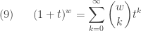
For convenience, we let 


where 
With the more relaxed notion of binomial coefficient, the probability function in 

Whenever r in 
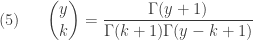
The following alternative parametrization of the negative binomial distribution is also useful.

The parameters in this alternative parametrization are r and 

________________________________________________________________________
What is negative about the negative binomial distribution?
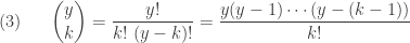
What is negative about this distribution? What is binomial about this distribution? The name is suggested by the fact that the binomial coefficient in

The calculation in 
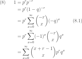
In 


For a detailed discussion of (8) with all the details worked out, see the post called Deriving some facts of the negative binomial distribution.
________________________________________________________________________
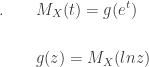
The Generating Function
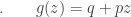
By definition, the following is the generating function of the negative binomial distribution, using :

where

As a result, the moment generating function of the negative binomial distribution is:
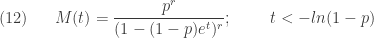
For a detailed discussion of (12) with all the details worked out, see the post called Deriving some facts of the negative binomial distribution.
________________________________________________________________________
Independent Sum
One useful property of the negative binomial distribution is that the independent sum of negative binomial random variables, all with the same parameter 


Note that the generating function of an independent sum is the product of the individual generating functions. The following shows that the product of the individual generating functions is of the same form as 
________________________________________________________________________

Mean and Variance
The mean and variance can be obtained from the generating function. From 


Note that 


________________________________________________________________________
The Poisson-Gamma Mixture
One important application of the negative binomial distribution is that it is a mixture of a family of Poisson distributions with Gamma mixing weights. Thus the negative binomial distribution can be viewed as a generalization of the Poisson distribution. The negative binomial distribution can be viewed as a Poisson distribution where the Poisson parameter is itself a random variable, distributed according to a Gamma distribution. Thus the negative binomial distribution is known as a Poisson-Gamma mixture.
In an insurance application, the negative binomial distribution can be used as a model for claim frequency when the risks are not homogeneous. Let 


Suppose that 


Then the joint density of

The unconditional distribution of 
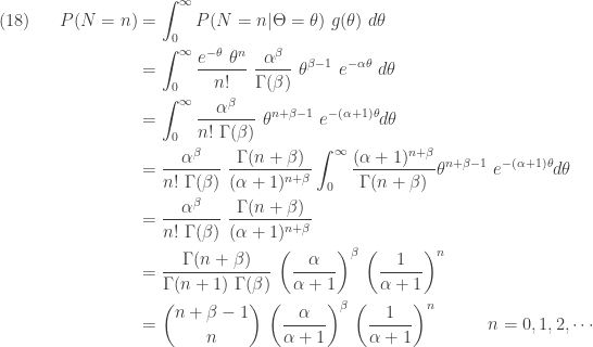
Note that the integral in the fourth step in 


The variance of the negative binomial distribution is greater than the mean. In a Poisson distribution, the mean equals the variance. Thus the unconditional distribution of
________________________________________________________________________
The Poisson Distribution as Limit of Negative Binomial
There is another connection to the Poisson distribution, that is, the Poisson distribution is a limiting case of the negative binomial distribution. We show that the generating function of the Poisson distribution can be obtained by taking the limit of the negative binomial generating function as 
In this section, we use the negative binomial parametrization of
![\displaystyle \begin{aligned}(19) \ \ \ \ \ \ &E(X)=\frac{r}{\alpha} \\&\text{ }\\&Var(X)=\frac{\alpha+1}{\alpha} \ \frac{r}{\alpha}=\frac{r(\alpha+1)}{\alpha^2} \\&\text{ } \\&g(z)=\frac{1}{[1-\frac{1}{\alpha}(z-1)]^r} \ \ \ \ \ \ \ z<\alpha+1 \end{aligned}](https://s0.wp.com/latex.php?latex=%5Cdisplaystyle+%5Cbegin%7Baligned%7D%2819%29+%5C+%5C+%5C+%5C+%5C+%5C+%26E%28X%29%3D%5Cfrac%7Br%7D%7B%5Calpha%7D+%5C%5C%26%5Ctext%7B+%7D%5C%5C%26Var%28X%29%3D%5Cfrac%7B%5Calpha%2B1%7D%7B%5Calpha%7D+%5C+%5Cfrac%7Br%7D%7B%5Calpha%7D%3D%5Cfrac%7Br%28%5Calpha%2B1%29%7D%7B%5Calpha%5E2%7D+%5C%5C%26%5Ctext%7B+%7D+%5C%5C%26g%28z%29%3D%5Cfrac%7B1%7D%7B%5B1-%5Cfrac%7B1%7D%7B%5Calpha%7D%28z-1%29%5D%5Er%7D+%5C+%5C+%5C+%5C+%5C+%5C+%5C+z%3C%5Calpha%2B1+%5Cend%7Baligned%7D&bg=ffffff&fg=333333&s=0&c=20201002)
Let r goes to infinity and 

![\displaystyle (20) \ \ \ \ \ \lim \limits_{r \rightarrow \infty} [1-\frac{\mu}{r}(z-1)]^{-r}=e^{\mu (z-1)}](https://s0.wp.com/latex.php?latex=%5Cdisplaystyle+%2820%29+%5C+%5C+%5C+%5C+%5C+%5Clim+%5Climits_%7Br+%5Crightarrow+%5Cinfty%7D+%5B1-%5Cfrac%7B%5Cmu%7D%7Br%7D%28z-1%29%5D%5E%7B-r%7D%3De%5E%7B%5Cmu+%28z-1%29%7D&bg=ffffff&fg=333333&s=0&c=20201002)
The right-hand side of 

![\displaystyle \begin{aligned}(21) \ \ \ \ \ \lim \limits_{r \rightarrow \infty} [1-\frac{\mu}{r}(z-1)]^{-r}&=\lim \limits_{r \rightarrow \infty} e^{\displaystyle \biggl(ln[1-\frac{\mu}{r}(z-1)]^{-r}\biggr)} \\&=\lim \limits_{r \rightarrow \infty} e^{\displaystyle \biggl(-r \ ln[1-\frac{\mu}{r}(z-1)]\biggr)} \\&=e^{\displaystyle \biggl(\lim \limits_{r \rightarrow \infty} -r \ ln[1-\frac{\mu}{r}(z-1)]\biggr)} \end{aligned}](https://s0.wp.com/latex.php?latex=%5Cdisplaystyle+%5Cbegin%7Baligned%7D%2821%29+%5C+%5C+%5C+%5C+%5C+%5Clim+%5Climits_%7Br+%5Crightarrow+%5Cinfty%7D+%5B1-%5Cfrac%7B%5Cmu%7D%7Br%7D%28z-1%29%5D%5E%7B-r%7D%26%3D%5Clim+%5Climits_%7Br+%5Crightarrow+%5Cinfty%7D+e%5E%7B%5Cdisplaystyle+%5Cbiggl%28ln%5B1-%5Cfrac%7B%5Cmu%7D%7Br%7D%28z-1%29%5D%5E%7B-r%7D%5Cbiggr%29%7D+%5C%5C%26%3D%5Clim+%5Climits_%7Br+%5Crightarrow+%5Cinfty%7D+e%5E%7B%5Cdisplaystyle+%5Cbiggl%28-r+%5C+ln%5B1-%5Cfrac%7B%5Cmu%7D%7Br%7D%28z-1%29%5D%5Cbiggr%29%7D+%5C%5C%26%3De%5E%7B%5Cdisplaystyle+%5Cbiggl%28%5Clim+%5Climits_%7Br+%5Crightarrow+%5Cinfty%7D+-r+%5C+ln%5B1-%5Cfrac%7B%5Cmu%7D%7Br%7D%28z-1%29%5D%5Cbiggr%29%7D+%5Cend%7Baligned%7D&bg=ffffff&fg=333333&s=0&c=20201002)
We now focus on the limit in the exponent.
![\displaystyle \begin{aligned}(22) \ \ \ \ \ \lim \limits_{r \rightarrow \infty} -r \ ln[1-\frac{\mu}{r}(z-1)]&=\lim \limits_{r \rightarrow \infty} \frac{ln(1-\frac{\mu}{r} (z-1))^{-1}}{r^{-1}} \\&=\lim \limits_{r \rightarrow \infty} \frac{(1-\frac{\mu}{r} (z-1)) \ \mu (z-1) r^{-2}}{r^{-2}} \\&=\mu (z-1) \end{aligned}](https://s0.wp.com/latex.php?latex=%5Cdisplaystyle+%5Cbegin%7Baligned%7D%2822%29+%5C+%5C+%5C+%5C+%5C+%5Clim+%5Climits_%7Br+%5Crightarrow+%5Cinfty%7D+-r+%5C+ln%5B1-%5Cfrac%7B%5Cmu%7D%7Br%7D%28z-1%29%5D%26%3D%5Clim+%5Climits_%7Br+%5Crightarrow+%5Cinfty%7D+%5Cfrac%7Bln%281-%5Cfrac%7B%5Cmu%7D%7Br%7D+%28z-1%29%29%5E%7B-1%7D%7D%7Br%5E%7B-1%7D%7D+%5C%5C%26%3D%5Clim+%5Climits_%7Br+%5Crightarrow+%5Cinfty%7D+%5Cfrac%7B%281-%5Cfrac%7B%5Cmu%7D%7Br%7D+%28z-1%29%29+%5C+%5Cmu+%28z-1%29+r%5E%7B-2%7D%7D%7Br%5E%7B-2%7D%7D+%5C%5C%26%3D%5Cmu+%28z-1%29+%5Cend%7Baligned%7D&bg=ffffff&fg=333333&s=0&c=20201002)
The middle step in 

________________________________________________________________________
Reference
- Klugman S.A., Panjer H. H., Wilmot G. E. Loss Models, From Data to Decisions, Second Edition., Wiley-Interscience, a John Wiley & Sons, Inc., New York, 2004
________________________________________________________________________


 . Thus the parameter
  , the following shows that
 (see
(see ![\displaystyle \begin{aligned}(2) \ \ \ \ \ &E(X)=g'(1)=\alpha \\&\text{ } \\&E[X(X-1)]=g^{(2)}(1)=\alpha^2 \\&\text{ } \\&Var(X)=E[X(X-1)]+E(X)-E(X)^2=\alpha^2+\alpha-\alpha^2=\alpha \end{aligned}](https://s0.wp.com/latex.php?latex=%5Cdisplaystyle+%5Cbegin%7Baligned%7D%282%29+%5C+%5C+%5C+%5C+%5C+%26E%28X%29%3Dg%27%281%29%3D%5Calpha+%5C%5C%26%5Ctext%7B+%7D+%5C%5C%26E%5BX%28X-1%29%5D%3Dg%5E%7B%282%29%7D%281%29%3D%5Calpha%5E2+%5C%5C%26%5Ctext%7B+%7D+%5C%5C%26Var%28X%29%3DE%5BX%28X-1%29%5D%2BE%28X%29-E%28X%29%5E2%3D%5Calpha%5E2%2B%5Calpha-%5Calpha%5E2%3D%5Calpha+%5Cend%7Baligned%7D&bg=ffffff&fg=333333&s=0&c=20201002)

 in a binomial distribution is large and the probability of success
  and the variance is
  . When
  is close to 1 and the binomial variance is approximately
  . Whenever the mean of a discrete distribution is approximately equaled to the mean, the Poisson approximation is quite good. As a rule of thumb, we can use Poisson to approximate binomial if
  and
and  .
. and
and  . So we use the Poisson distribution with
 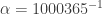 . The following is an estimate using the Poisson distribution.
 , then the independent sum
  has a Poisson distribution with parameter
  . One way to see this is that the product of Poisson generating functions has the same general form as
  and
and  , respectively. Then the number of “no purchase” customers and the number of “purchase” customers are independent Poisson random variables with parameters
  and
and  , respectively. For more details on the splitting of Poisson, see
  where
where 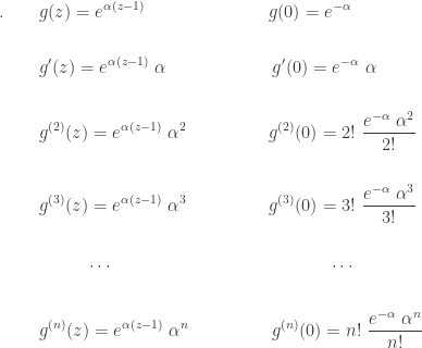
 at each order is a multiple of a Poisson probability. Thus the Poisson distribution is coded by the function
  is a random variable that takes only nonegative integer values with the probability function given by
 , .
, .
 .
.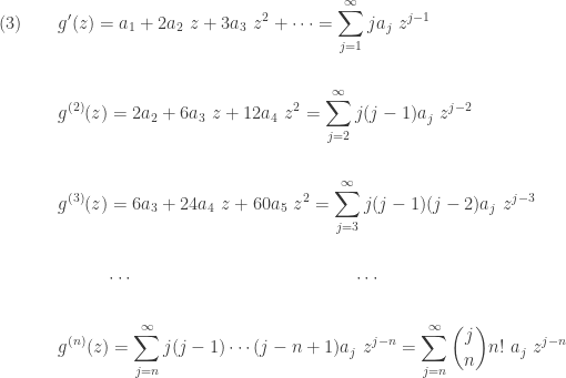
 above, all the terms vanishes except for the constant term. We have:
![\displaystyle \begin{aligned}(5) \ \ \ \ \ \ &g'(1)=0 \ a_0+a_1+2 a_2+3 a_3+\cdots=\sum \limits_{j=0}^\infty j a_j=E(X) \\&\text{ } \\&g^{(2)}(1)=0 a_0 + 0 a_1+2 a_2+6 a_3+ 12 a_4+\cdots=\sum \limits_{j=0}^\infty j (j-1) a_j=E[X(X-1)] \\&\text{ } \\&E(X)=g'(1) \\&\text{ } \\&E(X^2)=g'(1)+g^{(2)}(1) \end{aligned}](https://s0.wp.com/latex.php?latex=%5Cdisplaystyle+%5Cbegin%7Baligned%7D%285%29+%5C+%5C+%5C+%5C+%5C+%5C+%26g%27%281%29%3D0+%5C+a_0%2Ba_1%2B2+a_2%2B3+a_3%2B%5Ccdots%3D%5Csum+%5Climits_%7Bj%3D0%7D%5E%5Cinfty+j+a_j%3DE%28X%29+%5C%5C%26%5Ctext%7B+%7D+%5C%5C%26g%5E%7B%282%29%7D%281%29%3D0+a_0+%2B+0+a_1%2B2+a_2%2B6+a_3%2B+12+a_4%2B%5Ccdots%3D%5Csum+%5Climits_%7Bj%3D0%7D%5E%5Cinfty+j+%28j-1%29+a_j%3DE%5BX%28X-1%29%5D+%5C%5C%26%5Ctext%7B+%7D+%5C%5C%26E%28X%29%3Dg%27%281%29+%5C%5C%26%5Ctext%7B+%7D+%5C%5C%26E%28X%5E2%29%3Dg%27%281%29%2Bg%5E%7B%282%29%7D%281%29+%5Cend%7Baligned%7D&bg=ffffff&fg=333333&s=0&c=20201002)
![g^{(n)}(1)=E[X(X-1) \cdots (X-(n-1))]](https://s0.wp.com/latex.php?latex=g%5E%7B%28n%29%7D%281%29%3DE%5BX%28X-1%29+%5Ccdots+%28X-%28n-1%29%29%5D&bg=ffffff&fg=333333&s=0&c=20201002) . Thus the higher moment
. Thus the higher moment  can be expressed in terms of
  and
and  where
where  .
. , i.e.,
  . This provides a way to define the generating function for random variables that may take on values outside of the nonnegative integers. The following is a more general definition of the generating function of the random variable
  where the expectation exists.
 be independent random variables with generating functions
  , respectively. Then the generating function of
 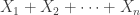 is given by the product
  .
.

 . The following is the binomial expansion:
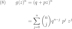

 , we have
 is that of a binomial distribution. Since the probability distribution of a random variable is uniquely determined by its generating function, the independent sum of Bernoulli distributions must ave a Binomial distribution.
 , respectively. Then the independent sum
  , the generating function of
 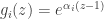 . The key to the proof is that the product of the
  has the same general form as the individual
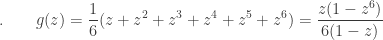
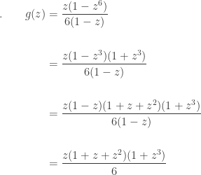
 be the sum of the 4 rolls. Then the generating function of
  is
is 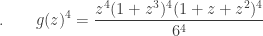
 to
to  . To find these probabilities, we simply need to decode the generating function
  . For example, to find
  , we need to find the coefficient of the term
  in the polynomial
 ,
,  ,
,  . Thus we have:
 , decode the probabilities from
  on all real numbers
  for which the expected value exists. The moments can be computed more directly using an mgf. From the theory of mathematical analysis, it can be shown that if
  exists on some interval
  , then the derivatives of
  . Furthermore, it can be show that
  .
.