The problem of points

There are two celebrated problems in probability that originated from the French professional gambler Chevalier de Méré (1607-1684). The problems were solved jointly by Blaise Pascal (1623-1662) and Pierre de Fermat (1601-1665) in a series of letters. The ideas discussed in these letters were often credited with having started probability theory. In a previous post, we discuss one of the problems posed by Chevalier de Méré to Pascal (the dice problem). In this post, we discuss the second problem – the problem of points.

___________________________________________________________________________

Describing the Problem

Here’s a description of the famous problem of points. Two players play a game of chance with the agreement that each player puts up equal stakes and that the first player who wins a certain number of rounds (or points) will collect the entire stakes. Suppose that the game is interrupted before either player has won. How do the players divide the stakes fairly?

It is clear that the player who is closer to winning should get a larger share of the stakes. Since the player who had won more points is closer to winning, the player with more points should receive a larger share of the stakes. How do we quantify the differential?

To describe the problem in a little more details, suppose that two players, A and B, play a series of points in a game such that player A wins each point with probability $p$ and that player B wins each point with probability $1-p$ . The first player to win $T$ points wins the game. Suppose that the game is stopped for some reason. At the time of stopping, player A has won $a$ points and player B has won $b$ points with $a<T$ and $b<T$ . How do they divide the stakes? Note that the pot is contributed equally by the two players.

In attacking the problem, Pascal’s idea is that the share of the stakes that is received by a player should be proportional to his/her probability of winning if the game were to continue at the point of stopping. Let’s explore this idea by looking at examples.

___________________________________________________________________________

Looking at the Problem thru Examples

The following examples are based on the following rule. Let’s say two players (A and B) play a series of points with equal probability of winning a point at each round. Each player puts up a stake of 32. The first player who wins four points take the entire stakes.

Example 1 (Fermat’s Approach)
Suppose that player A has won 2 points and player B has won one point right before the termination of the game. How can the stakes be divided fairly?

In the analysis, we assume that the game continues. Then player A needs 2 more points to win while player B needs 3 more points to win. We would like to calculate the probability that player A wins 2 points before player B winning 3 points. Consider the next 2 + 3 – 1 = 4 rounds (assuming one point per round). If player A wins at least 2 points in the next 4 rounds, player A win the game. The complement of this probability would be the probability that player B wins the game.

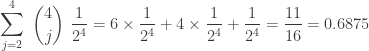
Let S (success) be the event that player A wins a point and let F (failure) be the event that player A loses a point (i.e. player B winning the point). Let’s write out all the outcomes of playing 4 points (this was the approach of Fermat). There are 16 such outcomes.

$\begin{array}{rrrrrr} 1 & SSSS & * & & \text{ } & \\ 2 & SSSF & * & & \text{ } & \\ 3 & SSFS & * & & \text{ } & \\ 4 & SSFF & * & & \text{ } & \\ 5 & SFSS & * & & \text{ } & \\ 6 & SFSF & * & & \text{ } & \\ 7 & SFFS & * & & \text{ } & \\ 8 & SFFF & \text{ } & & \text{ } & \\ 9 & FSSS & * & & \text{ } & \\ 10 & FSSF & * & & \text{ } & \\ 11 & FSFS & * & & \text{ } & \\ 12 & FSFF & \text{ } & & \text{ } & \\ 13 & FFSS & * & & \text{ } & \\ 14 & FFSF & \text{ } & & \text{ } & \\ 15 & FFFS & \text{ } & & \text{ } & \\ 16 & FFFF & \text{ } & & \text{ } & \\ \end{array}$

Player A wins In eleven of the outcomes (the ones with asterisk). Note that there are at least 2 S’s in the outcomes with asterisk. Thus the probability of player A winning is 11/16 = 0.6875. At the time of stopping the game, player A has a 68.75% chance of winning (if the game were to continue). The share for player A is 0.6875 x 64 = 44.

The example demonstrates the approach taken by Fermat. He essentially converted the original problem of points into an equivalent problem, i.e. finding the probability of player A winning the game if the game were to continue. Then he used combinatorial methods to count the number of cases that result in player A winning. In this example, the additional four points that are to be played are fictitious moves (the moves don’t have to be made) but are useful for finding the solution. The only draw back in Fermat’s approach is that he used counting. What if the number of points involved is large?

Example 2 (Pascal’s Approach)
The specifics of the example are the same as in Example 1. The listing out all possible cases in Example 1 makes the solution easy to see. But if the number of points is large, then the counting could become difficult to manage. What we need is an algorithm that is easy to use and is easy to implement on a computer.

Pascal essentially had the same thinking as Fermat, i.e. to base the solution on the probability of winning if the game were to continue. Pascal also understood that the original problem of points is equivalent to the problem of playing an additional series of points. In this example, playing additional 2 + 3 – 1 = 4 points. As in Example 1, we find the probability that player A wins 2 or more points in this series of 4 points. Pascal’s way to find this probability was based on what are now known as the Pascal’s triangle and the binomial distribution. We would use the following modern day notation:

$\displaystyle \sum \limits_{j=2}^4 \ \binom{4}{j} \ \frac{1}{2^4}=6 \times \frac{1}{2^4}+4 \times \frac{1}{2^4}+\frac{1}{2^4}=\frac{11}{16}=0.6875$

Note that the above probability of 0.6875 is the probability of having at least 2 successes in 4 trials (with 0.5 probability of success in each trial). Anyone with a good understanding of the binomial distribution can carry out the calculation (or use software). Of course, this mathematical construct came from Pascal! To the contemporaries of Pascal and Fermat, this concept was definitely not commonplace.

Example 3
Suppose that player A has won 1 point and player B has won no point at the time of termination of the game. How can the prize money be divided fairly?

Based on the discussion of Example 1 and Example 2, player A needs to win at least 3 points to win the game and player B needs to win 4 or more points to win the game. The extended series of points would have 3 + 4 – 1 = 6 points. Player A then needs to win at least 3 points out of 6 points (at least 3 successes out of 6 trials). The following gives the probability of player A winning the extended series of plays.

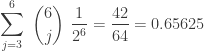
$\displaystyle \sum \limits_{j=3}^6 \ \binom{6}{j} \ \frac{1}{2^6}=\frac{42}{64}=0.65625$

With the total stakes being 64, the share for player A would be 64 x 42/64 = 42. The share for player B would be 22.

___________________________________________________________________________

General Discussion

We now discuss the ideas that are brought up in the examples. As indicated above, two players, A and B, contribute equally to the stakes and then play a series of points until one of them wins $T$ points. The probability that player A wins a round (one point in each round) is $p$ and the probability that player B wins a point is $1-p$ . Suppose that the game is stopped for some reason before either player has won. At the time of stopping, player A has won $a$ points and player B has won $b$ points with $a<T$ and $b<T$ . Let $n=T-a$ and $m=T-b$ . The key to solving the problem of points is to look at an extended play of $n+m-1$ points.

Here’s the great insight that came from Pascal and Fermat. They looked forward and not backward. They did not base the solution on the number of points that are already won. Instead, they focused on an extended series of points to determine the share of the winning. This additional play of points is “fictitious” but it helps clarify the process. In essence, they turned the original problem of points into a problem about this additional play of $n+m-1$ points.

The original problem is: what is the fair share for player A when the game is stopped prematurely with player A having won $a$ points and player B having won $b$ points? The equivalent problem is: what is the probability of player A winning at least $n$ points of the next $n+m-1$ points where $n=T-a$ and $m=T-b$ (assuming the game has not stopped). Let’s call this probability $P(n,m)$ . Let’s examine the setting of this probability. Each point is like a Bernoulli trial – either a success (player A winning it) or a failure (player B winning it). There are $n+m-1$ trials. The probability of success is $p$ in each trial. We wish to find the probability that are at least $n$ successes. What is being described is a binomial distribution. The probability being sought is:

$\displaystyle P(n,m)=\sum \limits_{j=n}^{n+m-1} \ \binom{n+m-1}{j} \ p^j \ (1-p)^{n+m-1-j} \ \ \ \ \ \ \ \ \ \ \ \ \ \ \ \ \ \ \ \ \ \ (1)$

where $n=T-a$ , $m=T-b$ and that $a$ is the number of points won by player A and $b$ is the number of points won by player B at the time the game is terminated.

The probability $P(n,m)$ is the probability of player A winning the game if the game were to continue at the point of termination. This probability $P(n,m)$ is the proportion of the stakes that would be awarded to player A. Of course, the proportion that should be awarded to player B would be $1-P(n,m)$ . The quantity $P(n,m)$ can be obtained from the given parameters and by using any software that has a function for the binomial distribution.

The problem of points seems to have an easy solution since the answer $P(n,m)$ is so accessible. Any one who understands the binomial distribution can comprehend. It is also easy to compute probabilities for a binomial distribution using calculator or software. One thing to keep in mind is that the solution looks accessible now because of the tools and concepts that came from trails blazed by Pascal and Fermat (and because of the computing tools that we have). Tools and concepts such as Pascal’s triangle and binomial distribution were unknown to people at the time of Pascal and Fermat.

___________________________________________________________________________

Working Backward

For us, the calculation in $(1)$ is easily done using calculator or software. Pascal did not calculate $P(n,m)$ directly and instead perform the calculation backward by using the following formula.

$P(n,m)=p \times P(n-1,m)+(1-p) \times P(n,m-1) \ \ \ \ \ \ \ \ \ \ \ \ \ \ \ \ \ \ \ \ \ \ (2)$

The formula can be derived mathematically. But doing that is not necessary. The quantity $P(n,m)$ is the probability that player A will win $n$ points before player B winning $m$ points. We can derive the above formula by conditioning on the outcome of the first point. The quantity $P(2,3)$ is calculated in Example 1 and Example 2. It is the average of two similar probabilities with smaller parameters.

$P(2,3)=\frac{1}{2} \times P(1,3)+\frac{1}{2} \times P(2,2)$

Based on the recursive formula in $(1)$ , Pascal built up the answer backward, similar to the way a computer program is written. In fact, this recursive approach allows us to solve not just for one scenario, but for all the scenarios in a game of $T$ points.

Example 4
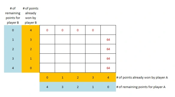
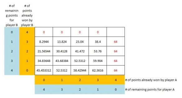
We now revisit the problem in Examples 1 and 2. Recall that the game is to play for 4 points, i.e. the first player winning 4 points collects the entire stakes of 64 (32 is contributed by each player). Each player earns a point with probability 0.5. We now show how to divide the stakes when the game is stopped at every possible stopping point.

The following diagram (Figure 1) shows the table for the share awarded to player A. The table is empty except for the top row and rightmost column (the numbers in red). The number 64 shown in the last column would be the amount awarded to player A because player A has won 4 points. The number 0 in the top means that player B has won 4 games. So player A gets nothing. Note that the bottom row highlighted in orange shows the numbers of points that have been won player A. The bottom row highlighted in blue shows the remaining points that player A needs to win in order to win the entire stakes (these are the fictitious points). Similarly, the columns highlighted in orange and blue on the left show the same information for player B.

Figure 1 – The share of the stakes awarded to player A
problem-of-points-by-table-1a

Now, we can use the recursive formula in $(1)$ to fill the table. Basically each cell is the average of the number above it and the number to the right. The parameter $n$ in $P(n,m)$ is a number in the blue row. The parameter $m$ in $P(n,m)$ is a number in the blue column. The following shows the results.

Figure 2 – The share of the stakes awarded to player A
problem-of-points-by-table-2a

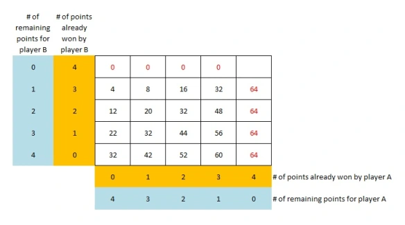
For example, when player A has won 2 points and player B has won 1 point, the share for player A is 44 (the average of 32 and 56), the same answer as in Example 1 and Example 2. When player A has won 2 points and player B as won 2 points, both players are in equally competitive positions. Then each player gets 32. When player A has won 2 points and player B as won 3 points, the share for player A is 16 (the average of 0 and 32).

Essentially the formula in $(2)$ is the idea of using smaller steps rather than the entire extended play of $n+m-1$ points. This idea of smaller steps was preferred by Pascal. At the point where player A needs $n$ more points to win and player B needs $m$ more points to win, the idea is to play one more point. Suppose that the players know the awards to the two players after one more round. Then they should split the difference between the future awards. The calculation should begin at the point where each player only needs one more point to win (the cell with 32 in Figure 2). In that cell, we know the awards after one additional round. Taking the average of 0 and 64 gives 32. From that cell, we move down and move left on the table. Keep repeating the process until the entire table is filled in.

There is a way to tweak the table approach to work for unequal winning probability of a point. Let’s say the probability of player A winning a point is 0.6. Then the probability of player B winning a point is 0.4. The value of a given cell in the table would be the weighted average of the cell on the right (0.6 weight) with the cell above it (0.4 weight). When we know the results from playing one more round, we assign 0.6 to the result of player A winning and 0.4 to the result of player B winning. The following table shows the results.

Figure 3 – The share of the stakes awarded to player A (with 0.6 weight)
problem-of-points-by-table-3a

The direct formula $(1)$ or the table approach using the recursive formula $(2)$ can be easily programmed in a computer. For Pascal, the table approach is a very attractive option since the calculation can be built up from lower parameter values. In the above configuration, simply fill in the right column (the entire stakes going to player A) and the top row (player A getting nothing). Then the remaining cells are obtained by weighted average as described in formula $(2)$ .

We present one more example.

Example 5
Suppose that player B is a casino and player A is a visitor at the casino playing for 12 points. The house edge is 2% so that the probability of player A winning a round is 0.48. If player A desires to leave after player A has won 9 points and the house has won 6 points, what is the proportion of the stakes that should be awarded to player A?

Playing for 12 points, player A needs 3 more points to win and the house needs 6 more points to win. So we need to analyze an extended play of 3 + 6 – 1 = 8 points. For player A to win the extended play, he needs to win at least 3 points.

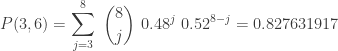
$\displaystyle P(3,6)=\sum \limits_{j=3}^8 \ \binom{8}{j} \ 0.48^j \ 0.52^{8-j}=0.827631917$

The answer can be obtained by computing each term in the sum (from $j=3$ to $j=8$ ). Another way is to use the BINOMDIST function in Excel as follows:

= 1-BINOMDIST(2, 8, 0.48, TRUE) = 1-0.172368083 = 0.827631917

Based on the fair division method discussed in this blog post, player A deserves 82.76% of the stakes.

___________________________________________________________________________

Remarks

In their correspondence, Pascal and Fermat came up with convincing and consistent solution to the problem of points. The earlier solutions to the problem of points were not satisfactory (to all concerned) and are sometimes inconsistent. Division of stakes only basing on the numbers points that have been won may produce extreme results. For example, if player A has won 1 point and player B has won no points, then player A would get the entire stakes. For the game described in Figure 2, for the same scenario, player A gets 42 out of 64 (42 / 64 = 0.65625), which is far from 100%.

For more detailed information on the history of the problem of points, see “A History of Mathematics” by Victor J. Katz.

___________________________________________________________________________
$\copyright \ 2016 \text{ by Dan Ma}$

9 thoughts on “The problem of points”

Pingback: When a gambler asked a mathematician for help | A Blog on Probability and Statistics
Pingback: Every character is known but password is hard to crack | A Blog on Probability and Statistics
Pingback: Five probability problems to help us think better | Math in the Spotlight
Pingback: The Dice Problem – Daniel Ma
Pingback: Seminer Konuları – Boğaziçi Üniversitesi Matematik Topluluğu
Pingback: Elo and EloBeta models in snooker | Smart Solution 4.0
Andrew V Showen on September 11, 2018 at 7:55 pm said:

I’m not a mathematician, but I do play games and I’m pretty good with math. But the solution to this problem troubles me because it makes no sense in the real world. When I tried to solve this problem, I used the Fermat method, laying out the possible outcomes as you have (SSSS, SSSF, SSFS, SSFF). However, in all of these 4 of 16 examples, the game ends after the second S (SS). This there is never any event in the real world that meets the description SSSF, SSFS, or SSFF), because the game stops. I do not understand why an event that will never happen — SSSF, SSFS, or SSFF) is assigned a probability greater than zero. If the game stops upon the occurrence of SS, then why aren’t SSSS, SSSF, SSFS, or SSFF treated as the same event, all of which have a single combined probability? In my analysis, SS xx was a single event; SFSx was a single event; FSSx was a single event.

On further reflection, I realized that if the probability of s =.5, then the probability of ss =.25. The probability of each of the ssxx events is .0625, so the probability of the ssxx events in sum is also .25. I presume this is not coincidence.

Still, my question remains: what is the justification for treating SSFF, SSSF, and SSFS as events with a probability that is not zero. I understand that IF one were to toss 4 coins, the result would be p=.0625, but this is like the gambler’s ruin fallacy, where trials 3 and 4 are never reached because the gambler runs out of money before the house does, and gets thrown out in the alley before reaching trial 3 and 4.

Reply ↓
- Stefan Weber on February 22, 2019 at 8:36 am said:
  
  Not all outcomes are actually possible (like SSFS, as you mentioned). Out of the 16 outcomes only 10 are possible and player A would win in 6 out of these 10 (60% win probability??) – instead of 11 out of 16 (68.75% win probability!!).
  But also not all “cases of success” for player A are possible but they get counted anyway. In combination, this results in a win probability of 68.75%.
  
  Now, the reason is that not all “cases of success” for player A have the same probability of happening. Therefore, if we are only to count the possible outcomes, we have to weigh the number of “cases of success” by the probability of each of these cases. Example:
  
  SS 25% –> 50%*50% = 0.5^2
  SFS 12.5% –> 0.5^3
  SFFS 6.25% –> 0.5^4
  FSS 12.5% –> 0.5^3
  FSFS 6.25% –> 0.5^4
  FFSS 6.25% –> 0.5^4
  =68.75%
  
  SFFF 6.25% –> 0.5^4
  FSFF 6.25% –> 0.5^4
  FFSF 6.25% –> 0.5^4
  FFF 12.5% –> 0.5^3
  =31.25%
  
  When you allow all combinations (even not possible ones like SSFS) you automatically assign each combination the same probability and can, thus, simply add up all successful combinations (without weighing by case probability).
  
  Reply ↓
ankitcreates on August 18, 2019 at 12:16 am said:

The explanation of the problem in the letters is very beautifully put forward by the author. Thank you so much !!

Reply ↓