Bayes’ formula gives better perspective on medical testing

Suppose that a patient is to be screened for a certain disease or medical condition. There are two important questions at the outset. How accurate is the screen or test? For example, at the outset, what is the probability of the test giving the correct result? The second question: once the patient obtains the test result (positive or negative), how reliable is the result? These two questions seem one and the same. Confusing these two questions as the same is a common misconception. Sometimes even medical doctors can get it wrong. This post demonstrates how to sort out these questions using Bayes’ formula or Bayes’ theorem.

Example

Before a patient is screened, a relevant question is on the accuracy of the test. Once the test result comes back, an important question is on whether positive result means having the disease and negative result means healthy. Here’s the two questions that are of interest:

• What is the probability of the test giving a correct result, positive for someone with the disease and negative for someone who is healthy?
• Once the test result is back, what is the probability that the test result is correct? More specifically, if a patient is tested positive, what is the probability that the patient has the disease? If a patient is tested negative, what is the probability that the patient is healthy?

Both questions involve conditional probabilities. In fact, the conditional probabilities in the second question are the reverse of the ones in the first question. To illustrate, we use the following example.

Example. Suppose that the prevalence of a disease is 1%. This disease has no particular symptoms but can be screened by a medical test that is 90% accurate. This means that the test result is positive about 90% of the times when it is applied on patients who have the disease and that the test result is negative about 90% of the time when it is applied on patients who do not have the disease. Suppose that you take the test and the test shows a positive result. Then the burning question is: how likely is it that you have the disease? Similarly, how likely is it that the patient is healthy if the test result is negative?

The accuracy of the test is 90% (0.90 as a probability). Since there is a 90% chance the test works correctly, if the patient has the disease, there is a 90% chance that the test will come back positive and if the patient is healthy, there is a 90% chance the test will come back negative. If a patient tested positive, wouldn’t it mean that there is a 90% chance that the patient has the disease?

Note that the given number of 90% is for the conditional events: “if disease, then positive” and “if healthy, then negative.” The example asks for the probabilities for the reversed events – “if positive, then disease”and “if negative, then healthy.” It is a common misconception that the two probabilities are the same.

Tree Diagrams

Let’s use a tree diagrams to look at this problem in a systematic way. First let be the event that the patient being tested is healthy (does not have the disease in question) and let be the event that the patient being tested is sick (has the disease in question). Let denote the event that the test result is positive if the patient has the disease. Let denote the event that the test result is negative if the patient is healthy.

Then and . These two conditional probabilities are based on the accuracy of the test. These probabilities are in a sense chronological – the patient either is healthy or sick and then is being tested. The example asks for the conditional probabilities and , which are backward from the given conditional probabilities, and are also backward in a chronological sense. We call and forward conditional probabilities. We call and backward conditional probabilities. Bayes’ formula is a good way to compute the backward conditional probabilities. The following diagram shows the structure of the tree diagram.

Figure 1 – Structure of Tree Diagram

At the root of the tree diagram is a randomly chosen patient being tested. The first level of the tree shows the disease status (H or S). The events at the first level are unconditional events. The next level of the tree shows the test status (+ or -). Note that the test status is a conditional event. For example, the + that follows H is the event and the – that follows H is the event . The next diagram shows the probabilities that are in the tree diagram.

Figure 2 – Tree Diagram with Probabilities

The probabilities at the first level of the tree are the unconditional probabilities and , where is the prevalence of the disease. The probabilities at the second level of the tree are conditional probabilities (the probabilities of the test status conditional on the disease status). A path probability is the product of the probabilities in a given path. For example, the path probability of the first path is , which equals . Thus a path probability is the probability of the event “disease status and test status.” The next diagram displays the numerical probabilities.

Figure 3 – Tree Diagram with Numerical Probabilities

Figure 3 shows four paths – “H and +”, “H and -“, “S and +” and “S and -“. With , the sum of the four path probabilities is 1.0. These probabilities show the long run proportions of the patients that fall into these 4 categories. The path that is most likely is the path “H and -“, which happens 89.1% of the time. This makes sense since the disease in question is one that has low prevalence (only 1%). The two paths marked in red are the paths for positive test status. Thus . Thus about 10.8% of the patients being tested will show a positive result. Of these, how many of them actually have the disease?

In this example, the forward conditional probability is . As the tree diagrams have shown, the backward conditional probability is . Of all the positive cases, only 8.33% of them are actually sick. The other 91.67% are false positives. Confusing the forward conditional probability as the backward conditional probability is a common mistake. In fact, sometimes medical doctors got it wrong according to a 1978 article in New England Journal of Medicine. Though we are using tree diagrams to present the solution, the answer of 8.33% is obtained by the Bayes’ formula. We will discuss this in more details below.

According to Figure 3, . Of these patients, how many of them are actually healthy?

Most of the negative results are actual negatives. So there are very few false negatives. Once gain, the forward conditional probability is not to be confused with the backward conditional probability .

Bayes’ Formula

The result seems startling. Thus if a patient tested positive, there is only a slightly more than 8% chance that the patient actually has the disease! It seems that the test is not very accurate and seems to be not reliable. Before commenting on this result, let’s summarize the calculation implicit in the tree diagrams.

Though not mentioned by name, the above tree diagrams use the idea of Bayes’ formula or Bayes’ rule to reverse the forward conditional probabilities to obtain the backward conditional probabilities. This process has been discribed in this previous post.

The above tree diagrams describe a two-stage experiment. Pick a patient at random and the patient is either healthy or sick (the first stage in the experiment). Then the patient is tested and the result is either positive or negative (the second stage). A forward conditional probability is a probability of the status in the second stage given the status in the first stage of the experiment. The backward conditional probability is the probability of the status in the first stage given the status in the second stage. A backward conditional probability is also called a Bayes probability.

Let’s examine the backward conditional probability . The following is the definition of the conditional probability .

Note that two of the paths in Figure 3 have positive test results (marked with red). Thus is the sum of two quantities with . One of the quantities is for the case of the patient being healthy and the other is for the case of the patient being sick. With , and plugging in ,

The above is the Bayes’ formula in the specific context of a medical diagnostic test. Though a famous formula, there is no need to memorize it. If using the tree diagram approach, look for the two paths for the positive test results. The ratio of the path for “sick” patients to the sum of the two paths would be the backward conditional probability .

Regardless of using tree diagrams, the Bayesian idea is that a positive test result is explained by two causes. One is that the patient is healthy. Then the contribution to a positive result is . The other cause of a positive result is that the patient is sick. Then the contribution to a positive result is . The ratio of the “sick” cause to the sum total of the two causes is the backward conditional probability . However, a tree diagram is clearly a very handy device to clarify the Bayesian calculation.

Further Discussion of the Example

The calculation in Figure 3 is based on the prevalence of the disease of 1%, i.e. . The hypothetical disease in the example affects one person in 100. With being relatively small (just 8.33%), we cannot place much confidence on a positive result. One important point to understand is that the confidence on a positive result is determined by the prevalence of the disease in addition to the accuracy of the test. Thus the less common the disease, the less confidence we can place on a positive result. On the other hand, the more common the disease, the more confidence we can place on a positive result.

Let’s try some extreme examples. Suppose that we are to test for a disease that nobody has (think testing for ovarian cancer among men or prostate cancer among women). Then we would have no confidence on a positive test result. In such a scenario, all positives would be healthy people. Any healthy patient that receives a positive result would be called a false positive. Thus in the extreme scenario of a disease with 0% prevalence among the patients being tested, we do not have any confidence on a positive result being correct.

On the other hand, suppose we are to test for a disease that everybody has. Then it would then be clear that a positive result would always be a correct result. In such a scenario, all positives would be sick patients. Any sick patient that receives a positive test result is called a true positive. Thus in the extreme scenario of a disease with 100% prevalence, we would have great confidence on a positive result being correct.

Thus prevalence of a disease has to be taken into account in the calculation for the backward conditional probability . For the hypothetical disease discussed here, let’s look at the long run results of applying the test to 10,000 patients. The next tree diagram shows the results.

Figure 4 – Tree Diagram with 10,000 Patients

Out of 10,000 patients being tested, 100 of them are expected to have the disease in question and 9,900 of them are healthy. With the test being 90% accurate, about 90 of the 100 sick patients would show positive results (these are the true positives). On the other hand, there would be about 990 false positives (10% of the 9,900 healthy patients). There are 990 + 90 = 1,080 positives in total and only 90 of them are true positives. Thus is 90/1080 = 8.33%.

What if the disease in question has a prevalence of 8.33%? What would be the backward conditional probability assuming that the test is still 90% accurate?

With , there is a great deal more confidence on a positive result. With the test accuracy being the same (90%), the greater confidence is due to the greater prevalence of the disease. With being greater than 0.01, a greater portion of the positives would be true positives. The higher the prevalence of the disease, the greater the probability . Just to further illustrate this point, suppose the test for a disease has a 90% accuracy rate and the prevalence for the disease is 45%. The following calculation gives .

With the prevalence being 45%, the probability of a positive being a true positive is 88%. The calculation shows that when the disease or condition is widespread, a positive result should be taken seriously.

One thing is clear. The backward conditional probability is not to be confused with the forward conditional probability . Furthermore, it will not be easy to invert the forward conditional probability without using Bayes’ formula (either using the formula explicitly or using a tree diagram).

Bayesian Updating Based on New Information

The calculation shown above using the Bayes’ formula can be interpreted as updating probabilities in light of new information, in this case, updating risk of having a disease based on test results. With the hypothetical disease having a prevalence of 1% being discussed above, the initial risk is 1%. With one round of testing using a test with 90% accuracy, the risk is updated to 8.33%. For the patients who test positive in the first round of testing, the risk is raised to 8.33%. They can then go through a second round of testing using another test (but also with 90% accuracy). For the patients who test positive in the second round, the risk is updated to 45%. For the positives in the third round of testing, the risk is updated to 88%. The successive Bayesian calculation can be regarded as sequential updating of probabilities. Such updating would not be easy without the idea of the Bayes’ rule or formula.

Sensitivity and Specificity

The sensitivity of a medical diagnostic test is the ability to give correct results for the people who have the disease. Putting it in another way, the sensitivity is the true positive rate, which would be the percentage of sick people who are correctly identified as having the disease. In other words, the sensitivity of a test is the probability of a correct test result for the people with the disease. In our discussion, the sensitivity is the conditional forward probability .

The specificity of a medical diagnostic test is the ability to give correct results for the people who do not have the disease. The specificity is then the true negative rate, which would be the percentage of healthy people who are correctly identified as not having the disease. In other words, the specificity of a test is the probability of a correct test result for healthy people. In our discussion, the specificity is the conditional forward probability .

With the sensitivity being the conditional forward probability , the discussion in this post shows that the sensitivity of a test is not the same as backward conditional probability . The sensitivity may be 90% but the probability can be much lower depending on the prevalence of the disease. The sensitivity only tells us that 90% of the people who have the disease will have a positive result. It does not take into account of the prevalence of the disease (called the base rate). The above calculation shows that the rarer the disease (the lower the base rate), the lower the likelihood that a positive test result is a true positive. Likewise, the more common the disease, the higher the likelihood that a positive test result is a true positive.

In the example discussed here, both the sensitivity and specificity are 90%. This scenario is certainly ideal. In medical testing, the accuracy of a test for a disease may not be the same for the sick people and for the healthy people. For a simple example, let’s say we use chest pain as a criterion to diagnose a heart attack. This would be a very sensitive test since almost all people experiencing heart attack will have chest pain. However, it would be a test with low specificity since there would be plenty of other reasons for the symptom of chest pain.

Thus it is possible that a test may be very accurate for the people who have the disease but nonetheless identify many healthy people as positive. In other words, some tests have high sensitivity but have much lower specificity.

In medical testing, the overriding concern is to use a test with high sensitivity. The reason is that a high true positive rate leads to a low false negative rate. So the goal is to have as few false negative cases as possible in order to correctly diagnose as many sick people as possible. The trade off is that there may be a higher number of false positives, which is considered to be less alarming than missing people who have the disease. The usual practice is that a first test for a disease has high sensitivity but lower specificity. To weed out the false positives, the positives in the first round of testing will use another test that has a higher specificity.

2017 – Dan Ma

More about Monty Hall Problem

The previous post is on the Monty Hall Problem. This post adds to the discussion by looking at three pieces from New York Times. Anyone who is not familiar with the problem should read the previous post or other online resources of the problem.

The first piece describes a visit by John Tierney at the home of Monty Hall, who was the host of the game show Let’s Make a Deal, the show on which the Monty Hall Problem was loosely based. The visit took place in Beverly Hills back in 1991, one year after the firestorm caused by the publication of Monty Hall Problem by Marilyn vos Savant in Parade Magazine. The purpose of the visit is to obtain more confirmation that the counter intuitive answer (switching door) is correct and to get more insight about the game from Monty Hall himself.

Before discussing the visit, here’s the statement of Monty Hall Problem. The previous post actually uses five pictures to describe the problem.

“Suppose you’re on a game show, and you’re given the choice of three doors: Behind one door is a car; behind the others, goats. You pick a door, say No. 1, and the host, who knows what’s behind the other doors, opens another door, say No. 3, which has a goat. He then says to you, ‘Do you want to pick door No. 2?’ Is it to your advantage to take the switch?”

In front of Tierney, Monty Hall performed a simulation in his dining room. Monty Hall put three miniature cardboard doors on a table and represented the car with an ignition key. The goats were played by a package of raisins and a roll of Life Savers. Monty Hall conducted 10 rounds of the game as the contestant (John Tierney) tried the non-switching strategy. The result was that the contestant won four cars and six goats.

Then in the next 10 rounds, the contestant tried switching doors. The result was markedly different – the contestant won eight cars and two goats. The simulation gives strong indication that it is more advantageous to switch door.

The standard solution: with the switching door strategy, the contestant wins the car 2/3 of the time. On the other hand, the contestant only wins the car 1/3 of the time if he/she stick with the original pick.

It turns out that the optimal solution of switching door should come with a caveat, which is given in the previous post. The caveat is that the strategy of switching door works only if the moves of the game are determined by random chance – the contestant picks a door at random, then the host picks a door at random (if the contestant’s pick happens to be the winning door). After the choices are made at random, the host will be required to offer the chance to switch. Once all these conditions are met, the switching door strategy will be optimal.

The description in the preceding paragraph works like a computer program, in which all the rules are clear cut. There is no psychological factor involved. But Monty Hall did not run his show like a computer program. He sometimes did things that are meant to trick the contestants.

Month Hall did not always followed the standard assumptions. According to the NY Times piece, sometimes Monty Hall simply opened the contestant’s original pick (if it is a goat). So the picking a door showing a goat routine did not have to be done. Sometimes, he conned the contestant into switching door (if the contestant’s original door is a car), in which case, the switching strategy would have a zero chance of winning.

So there is psychological factor to consider in the actual Monty Hall game. The host may try to trick you into making a wrong move.

In fact, the statement of the problem given above (the same wording as in Marilyn vos Savant’s column) has a loop hole of sort. It did not explicitly make clear that the host will always open a door with a goat and then offer a switch. Monty Hall said, “if the host is required to open a door all the time and offer you a switch, then you should take the switch.” Furthermore, he said “but if he has the choice whether to allow a switch or not, beware. Caveat emptor. It all depends on his mood.” Here’s his advice, “if you can get me to offer you $5,000 not to open the door, take the money and go home.”

So the actual way in which the game is played may render the “academic” solution of the Monty Hall problem useless or meaningless. In any case, whenever the standard solution of Monty Hall Problem is given, the caveat should also be given. Indeed, if the game is played according to a random chances and if the contestant always switches door, then the company that hosts the game would lose too many cars! For financial reasons, they cannot run the show like clock work.

The second piece from NY Times is on the cognitive dissonance that some people experienced with the Monty Hall problem.

The third piece is a more recent discussion and is concerned with variations of the standard Monty Hall Problem. This piece consider tweaks to the basic game in two ways. The question: does each way of tweaking reduce the probability of the host losing a car? Or what is the probability of the host losing a car? Here’s the two tweaks.

First challenge: Suppose Monty Hall’s game show is losing money, and they want to tweak the game so they don’t lose the car as frequently. They announce to the audience that once you choose the door, the host will flip a fair coin to decide which of the other doors will be opened. If the car is behind the door that they open, you lose. If it is not behind the door that they open, you get to choose whether to stick with your door or to change to the other closed door. What do you do if that happens? And now, going into the game, assuming that the contestant behaves optimally, what is the probability that the game show will lose the car?

Second challenge: Now suppose that the game show gets even greedier, and secretly tweaks the game even more. But news of their tweaking is leaked, and the contestants find out that the host is actually using a weighted coin when they are determining which other door will be opened, and the coin is weighted such that the door with the car behind it will be opened by the host with ¾ probability. (When the car is behind the door that you choose initially, the host uses a fair coin to determine which of the other doors to open.) Now, if the door that they open doesn’t have the car behind it – should you stick with your original choice or should you switch? And, assuming that the contestant behaves optimally, did the nefarious game show succeed in reducing the probability that they lose the car?

In each tweak, the problem assumes that the contestant behaves optimally in the game. I suppose that means the contestant always switches door if the switching is possible. An even more interesting exercise would be to calculate the probability under the switching scenario and under the sticking scenario.

___________________________________________________________________________
2017 – Dan Ma

Monty Hall Problem

The post discusses the Monty Hall problem, a brain teaser and a classic problem in probability. The following 5 pictures describe the problem. Several simple solutions are presented.

___________________________________________________________________________

The Problem in Pictures

Figure 1

Figure 2

Figure 3

Figure 4

Figure 5

___________________________________________________________________________

Should You Switch?

Assuming that you, the contestant in the show, wants to win a car and not a goat, which door should you pick? Should you stick with your original pick of Door 1, or should you switch to Door 2? It is clear that had the game show host not intervened by opening another door, your chance of winning a car would be 1/3. Now that one door had been eliminated, you are faced with two doors, one being your original pick and another door. Would choosing one door out of two means your chance of winning the car is now 1/2? If this were the case, it would mean it does not matter whether you switch your choice or not. Enough people were reasoning in this same way that this problem stirred up a huge controversy back in 1990 when the problem was posed on Parade Magazine. More about that later. For now, let’s focus on the solution.

It is to your advantage to switch your choice. With switching, the probability of winning the car is 2/3, while the winning probability is 1/3 if you stick with the original choice. The rest of the post attempts to convince doubters that this is correct.

___________________________________________________________________________

The Problem to be Solved

The problem described by the 5 pictures above is based on the assumption that the contestant picks Door 1 and the host picks Door 3. The problem in the pictures is asking for the conditional probability of winning by switching given that the contestant picks Door 1 and the host picks Door 3. We solve a slightly different problem: what is the probability of winning a car if the contestant uses the “switch” strategy, which is the strategy of choosing the alternative door offered by the game show host. At the end, the first problem is also discussed.

The game involves selections of doors by the contestant and the host as well as by the staff who puts the prizes behind the three doors. It is important to point out that the manner in which the doors are chosen is important. Basically the doors have to be selected at random. For example, the staff of the game show selects the door with the car at random, the contestant selects his/her door at random, and the game show host select his/her door at random (in case that the door with car and the contestant’s door are the same). Under these assumptions, the best strategy is to switch. If the doors are not selected at random, the solution may not be the “switch” strategy.

___________________________________________________________________________

Simulation

An effective way to demonstrate that switching door is the optimal solution is through playing the game repeatedly. Let’s use a die to simulate 20 plays of the game. The simulation is done in 4 steps. In Steps 1 and 2, roll a fair die to select a door at random. If it turns up 1 or 2, then it is considered Door 1. If it turns up 3 or 4, then Door 2. If it turns up 5 or 6, then Door 3. In Step 3, the host also rolls a die to select a door if the door with car happens to be the same as the contestant’s choice.

In Step 1, the rolling of the die is to determine the prize (i.e. which door has the car). In Step 2, the rolling of the die is to determine the choice of door of the contestant. In Step 3, the host chooses a door based on Step 1 and Step 2. If the door with the car and the door chosen by the contestant are different, the host has only one choice. If the door with the car and the contestant’s door are identical, then the host will roll a die to choose a door. For example, if Door 1 is the door with the car and the door chosen by the contestant, then the host chooses Door 2 and Door 3 with equal probability (e.g. if the roll of the die is 1, 2 or 3, then choose Door 2, otherwise choose Door 3).

Step 1- Simulate the Doors with Car

Play	Door with Car
#1	1
#2	3
#3	3
#4	2
#5	2
#6	1
#7	1
#8	2
#9	1
#10	1
#11	2
#12	3
#13	1
#14	2
#15	2
#16	2
#17	3
#18	3
#19	1
#20	1

Step 2- Simulate the Doors Chosen by the Contestant

Play	Door with Car	Contestant’s Choice
#1	1	2
#2	3	1
#3	3	1
#4	2	3
#5	2	3
#6	1	2
#7	1	1
#8	2	3
#9	1	1
#10	1	2
#11	2	2
#12	3	2
#13	1	1
#14	2	2
#15	2	1
#16	2	2
#17	3	2
#18	3	3
#19	1	2
#20	1	3

Step 3- Simulate the Doors Chosen by the Host

Play	Door with Car	Contestant’s Choice	Host’s Choice
#1	1	2	3
#2	3	1	2
#3	3	1	2
#4	2	3	1
#5	2	3	1
#6	1	2	3
#7	1	1	2
#8	2	3	1
#9	1	1	3
#10	1	2	3
#11	2	2	1
#12	3	2	1
#13	1	1	3
#14	2	2	3
#15	2	1	3
#16	2	2	3
#17	3	2	1
#18	3	3	2
#19	1	2	3
#20	1	3	2

Step 4 – Contestant Makes the Switch

Play	Door with Car	Contestant’s Choice	Host’s Choice	Switched Door	Car/Goat
#1	1	2	3	1	Car
#2	3	1	2	3	Car
#3	3	1	2	3	Car
#4	2	3	1	2	Car
#5	2	3	1	2	Car
#6	1	2	3	1	Car
#7	1	1	2	3	Goat
#8	2	3	1	2	Car
#9	1	1	3	2	Goat
#10	1	2	3	1	Car
#11	2	2	1	3	Goat
#12	3	2	1	3	Car
#13	1	1	3	2	Goat
#14	2	2	3	1	Goat
#15	2	1	3	2	Car
#16	2	2	3	1	Goat
#17	3	2	1	3	Car
#18	3	3	2	1	Goat
#19	1	2	3	1	Car
#20	1	3	2	1	Car

There are 13 cars in Step 4. In 20 simulated plays of the game, the contestant wins 13 times using the switching strategy, significantly more than 50% chance of winning. Of course, if another simulation is performed, the results will be different. We perform 10 more simulations in Excel with 10,000 plays of the game in each simulation. The numbers of winnings in these simulations are:

10 More Simulations

Simulation	Number of Games	Number of Winning Games
#1	10,000	6,644
#2	10,000	6,714
#3	10,000	6,549
#4	10,000	6,692
#5	10,000	6,665
#6	10,000	6,687
#7	10,000	6,733
#8	10,000	6,738
#9	10,000	6,625
#10	10,000	6,735
Total	100,000	66,782

In each of the 10 simulations, the chance of winning a car is between 66% and 67% (by switching). In all of the 100,000 simulated games, the chance for winning a car by switching door is 66.782%. More and more simulations showing essentially the same results should give us confidence that the “switch” strategy increases the chance of winning and that the probability of winning is around 2/3.

If anyone who still thinks that switching does not make a difference, perform simulations of your own. It can be done by rolling a die as done here or by using computer generated random numbers. In fact, a computer simulation can produce tens of thousands or more plays. But anyone who does not trust computer simulations can simply generate 100 games by rolling the die. Simulations, when done according to the assumptions behind the game (the assumptions that the doors are selected at random), do not lie. In fact, many of the skeptics in the Monty Hall problem were convinced by simulations.

___________________________________________________________________________

Listing Out All Cases

Note that in Step 4 of the simulation, one pattern is clear about switching to the door offered by the host. The contestant will win a goat if his/her original choice of door happens to be the same as the door with the car. On the other hand, the contestant will win a car if his/her original choice happens to be different from the winning door. The observation is actually another explanation of the solution.

Let’s say the contestant picks Door 1 originally. There are three cases to consider since the winning door can be any one of the three door. Let’s look at what happens if the contestant switches door in each case.

The Three Cases for the Winning Door
Door 1 is Contestant’s Choice

The contestant wins 2 of the three cases by switching door. The contestant wins in only one of the cases if he/she were to stick with the original choice of door. The three cases are equally likely since the winning door is supposed to be randomly selected. So in the “switch” strategy, the probability of winning a car is 2/3.

___________________________________________________________________________

Looking at Two Diagrams

The solution in the previous section is a simple but correct solution. For anyone who thinks the solution is too simple, the following two diagrams can supplement the reasoning in the above simple solution.

Figure 6

In Figure 6, assume that the contestant picks Door 1, which as a 1/3 chance of winning a car. Then the other two doors as a group has a 2/3 chance of winning the car.

Figure 7

In Figure 7, the game show host opens a door with a goat (Door 3). The two doors of Door 2 and Door 3 as a group still has a 2/3 chance of winning a car. Since Door 3 is eliminated by the host, Door 3 now has zero chance of winning a car. So Door 2 has a 2/3 probability of winning the car. It is then advantageous for the contestant to switch door.

___________________________________________________________________________

Tree Diagram

Another way to view the problem is through a tree diagram. The idea is that such a tree diagram would capture the idea that the game show takes places in stages, e.g. the car is randomly placed behind one door, the contestant randomly picks one door, the host picks a door (randomly if required). The following diagram captures the entire random process.

Figure 8

Because the door is chosen at random, the probability at a branch is 1/3 if there are three branches at a decision point and the probability is 1/2 if there are two branches at any given node. Of course, if there is only one choice of a door, then the probability at the point is 1. There are 12 paths in the tree and each path probability is the product of all the individual probabilities in that path. At the right of the diagram, we compare the stay strategy and the switch strategy. With the stay strategy, the contestant wins in 6 of the paths. If using the switch strategy, the contestant wins in the other 6 paths. But the 6 paths with the switch strategy are twice as likely to happen.

___________________________________________________________________________

The Problem Described in the Pictures

The several solutions so far solve a general problem – if the contestant picks the door offered by the game show host, what is the probability of winning a car? In the pictures, the problem is: if the contestant picks Door 1 and the host picks Door 3, what is the winning probability for the contestant under the switch strategy? This is a conditional probability. Figure 8 has all the ingredients for the answer to this problem. In Figure 8, there are two paths in which the contestant picks Door 1 and the host picks Door 3. The following diagram shows these two paths with a check mark.

Figure 9

For one of these two paths, the car is behind Door 1 and for the other path, it is behind Door 2. The path with the car behind Door 2 is twice as likely as the one with the car behind Door 1. With the switching strategy, the path with the car behind Door 1 would lead to a goat (losing path) and the path with car behind Door 2 will lead to a car (winning path). The winning path is twice as likely. Thus the winning probability for the switch strategy is 2/3 if the contestant picks Door 1 and the host picks Door 3. Now this answer is the same as the answer for the general problem discussed previously. However, the conditional problem is a different problem.

___________________________________________________________________________

Remarks

The Monty Hall problem is loosely based on a real game show called Let’s Make a Deal. At one point in time, it was only a brain teaser as well as an academic problem (being discussed in statistics journals). In 1990, it appeared in a column by Marilyn vos Savant in Parade Magazine. In that column, vos Savant used the simple 3-case solution above to explain that the contestant should switch. The problem generated so many responses from angry readers, some of them had PhDs in math or statistics. Because of the ensuing controversy, the Monty Hall problem became a famous problem the world over. It is covered in many standard probability and statistics books and courses. Eventually some of those angry readers came to understand that the correct answer is the switch strategy. In fact, Paul Erdős, a famous and prolific mathematician in the 20th century, did not believe that switching is the correct answer. He remained unconvinced until someone showed him a computer simulation (see here).

Some psychologists asserted that the Monty Hall problem causes cognitive dissonance. As a result, the problem is confusing and even troubling to some people. See this article for the discussion.

The Monty Hall problem is all over the Internet. The Wikipedia entry on Monty Hall problem has more detailed information mathematically and in many other aspects. This article from Scientific American is also interesting.

___________________________________________________________________________
2017 – Dan Ma

The gambler’s ruin problem

This post discusses the problem of the gambler’s ruin. We start with a simple illustration.

Two gamblers, A and B, are betting on the tosses of a fair coin. At the beginning of the game, player A has 1 coin and player B has 3 coins. So there are 4 coins between them. In each play of the game, a fair coin is tossed. If the result of the coin toss is head, player A collects 1 coin from player B. If the result of the coin toss is tail, player A pays player B 1 coin. The game continues until one of the players has all the coins (or one of the players loses all his/her coins). What is the probability that player A ends up with all the coins?

Intuitively, one might guess that player B is more likely to win all the coins since B begins the game with more coin. For example, player A in the example has only 1 coin to start. Thus there is a 50% chance that he/she will lose everything on the first toss. On the other hand, player B has a cushion since he/she can afford to lose some tosses at the beginning.

___________________________________________________________________________

Simulated Plays of the Game

One way to get a sense of the winning probability of a player is to play the game repeatedly. Rather than playing with real money, why not simulate a series of coin tosses using random numbers generated in a computer? For example, the function =RAND() in Excel generates random numbers between 0 and 1. If the number is less than 0.5, we take it as a tail (T). Otherwise it is a head (H). As we simulate the coin tosses, we add or subtract to each player’s account accordingly. If the coin toss is a T, we subtract 1 from A and add 1 to B. If the coin toss is an H, we add 1 to A and subtract 1 from B. Here’s a simulation of the game.

In the first simulation, player A got lucky with 4 heads in 5 tosses. The following shows the next simulation.

Player A seems to be on a roll. Here’s the results of the next two simulated games.

Now player A loses both of these games. For good measure, we show one more simulation.

This one is a little more drawn out. Several tosses of tail in a row spells bad news for player A. When a coin is tossed long enough, there bounds to be some runs of tails. Since it is a fair coin, there bounds to be runs of head too, which benefit player A. Wouldn’t the runs of H cancel out the runs of T so that each player wins about half the time? To get an idea, we continue with 95 more simulations (to get a total of 100). Player A wins 23 of the simulated games and player B wins 77 of the games. So player A wins about 25% of the times. Note that A owns about 25% of the coins at the start of the game.

The 23 versus 77 in the 100 simulated games may be just due to luck for player B. We simulate 9 more runs of 100 games each (for a total of 10 runs with 100 games each). The following shows the results.

Ten Simulated Runs of 100 Games Each

The simulated runs fluctuate quite a bit. Player A wins any where from 19% to 34% of the times. The results are no where near even odds of winning for player A. In the 1,000 simulated games, player A wins 24.6% of the times, roughly identical to the player A’s share of the coins at the beginning. If the simulation is carried many more times (say 10,000 times or 100,000 times), the overall winning probability for player A would be very close to 25%.

___________________________________________________________________________

Gambler’s Ruin Problem

Here’s a slightly more general description of the problem of gambler’s ruin.

Gambler’s Ruin Problem

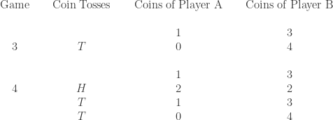
Two gamblers, A and B, are betting on the tosses of a fair coin. At the beginning of the game, player A has coins and player B has coins. So there are coins between them. In each play of the game, a fair coin is tossed. If the result of the coin toss is head, player A collects 1 coin from B. If the result of the coin toss is tail, player A pays B 1 coin. The game continues until one of the players has all the coins. What is the probability that player A ends up with all the coins? What is the probability that player B ends up with all the coins?

Solution: Gambler’s Ruin Problem

The long run probability of player A winning all the coins is .
The long run probability of player B winning all the coins is .

In other words, the probability of winning for a player is the ratio of the number of coins the player starts with to the total numbers of coins. Turning it around, the probability of a player losing all his/her coins is the ratio of the number of coins of the other player to the total number of coins. Thus the player with the fewer number of coins at the beginning has a greater chance of losing everything. Think a casino. Say, it has 10,000,000 coins. You, as a gambler, have 100 coins. Then you would have a 99.999% chance of losing all your coins.

The 99.999% chance of losing everything is based on the assumption that all bets are at even odds. This is certainly not the case in a casino. The casino enjoys a house edge. So the losing probabilities would be worse for a gambler playing in a casino.

___________________________________________________________________________

Deriving the Probabilities

We derive the winning probability for a more general case. The coin that is tossed does not have to be a fair coin. Let be the probability that the coin toss results in a head. Let . Suppose that there are coins initially between player A and player B.

Let be the probability that player A will own all the coins when player A starts the game with coins and player B starts with coins. On the other hand, let be the probability that player B will own all the coins when player A starts the game with coins and player B starts with coins.

The goal here is to derive expressions for both and for and to show that . The last point, though seems like common sense, is not entirely trivial. It basically says that the game will end in finite number of moves (it cannot go on indefinitely).

Another point to keep in mind is that we can assume and as well as and . In the following derivation, is the event that the first toss is a head and is the event that the first toss is a tail.

Let be the event that player A owning all the coins when player A starts the game with coins and player B starts with coins, i.e. . First condition on the outcome of the first toss of the coin.

Consider the conditional probabilities and . Note that . If the first toss is a head, then player A has coins and player B would have coins. At that point, the probability of player A owning all the coins would be the same as the probability of winning as if the game begins with player A having coins. Similarly, . Plug these into (1), we have:

Further derivation can be made on equation (2).

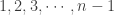Plugging in the values for produces the following equations.

Adding the first equations produces the following equations.

There are two cases to consider. Either or . The first case means and the second case means . The following is an expression for for the two cases.

The above two-case expression for is applicable for . Plugging into with gives the following expression for :

Plugging from (5) into (4) gives the following:

The expression for in (6) is applicable for . For the case of , the probability of player A owning all the coin is the ratio of the initial amount of coins of player A to the total number of coins, identical to what is stated in the previous section. Recall that is the probability that player B will end up owning all the coins when initially player A has coins and player B has coins. By symmetry, the following gives the expression for .

For the case , which is equivalent to , it is clear that . For the case , the following shows that .

The fact that shows that the gambling game discussed here has to end after certain number of plays and that it will not continue indefinitely.

___________________________________________________________________________

Further Discussion

The formulas derived here are quite profound, not to mention impactful and informative for anyone who gambles. More calculations and discussion can be found here in a companion blog on statistics.

___________________________________________________________________________
2017 – Dan Ma

Are digits of pi random?

What better way to celebrate Pi Day than to have a blog post on the digits of !

Giving pi as tips

The number is the ratio of the circumference of a circle to its diameter. It is an irrational number. This means that the decimal expansion of never ends and never repeats. Any decimal representation of with just a finite number of decimal places written out is an approximation.

In any calculation involving , the more decimal places, the more precise the computation will be. Approximations of used in computations can range from 3.14 to 3.14159 (for hand calculation), or from 3.141592654 to 3.14159265358979 (using calculator or software). In fact, the calculations involving performed in NASA use 15 or 16 significant digits (the last approximation cited has 15 significant digits).

As of the writing of this post, has been successfully calculated to over 22 trillions decimal places, or 22,459,157,718,361 decimal places to be exact (see here). If 15 or 16 digits are good enough for space travel, why the fascination with with billions and trillions or more digits? Why strive for more digits of than we will ever need for practical applications on Earth or in space?

Jumping on the pi band wagon could be all about pi mania. People had been fascinated with since antiquity. In our contemporary society, a day is set aside to celebrate the number pi. Actually two days are set aside – March 14 (3.14) and July 22 (based on 22/7 as an approximation), even though the first one is more well known than the second one. There are plenty of other well known special numbers. But I have never heard of a Natural Log Constant Day or Square Root of 2 Day.

There are indeed some special needs for that require billions or more digits. One is that is used in testing computer precision. The other is that digits of are sometimes used as random digits generator. Even such uses speak more of pi mania than the natural and intrinsic qualities of the pi since other special numbers can instead be used for these purposes.

Of course, as a number is not random. The digits are fixed and determined ahead of time. The first decimal place is always 1, the second decimal place is always 4 and so on. The third decimal place in the number could not be any digit other than 1. Instead, we should ask a different question.

Are the decimal digits of uniformly distributed? In other words, does every digit (from 0 to 9) in the decimal expansion of appear one-tenth of the time? Does every pair of digits appear one-hundredth of the time? Does every triple of digits in the decimal expansion of appear one-thousandth of the time and so on? If that is the case, we would say is a normal number in base 10.

The concept of normal number applies to other bases too. So if each digit in the binary expansion of a number appears half the time, and if each pair of binary digits (00, 01, 10 and 11) appear one-quarter of the time and so on, the number in question is called a normal number in base 2. In general, for a number to be a normal number in a given base, every sequence of possible digits in that base is equally likely to appear in the expansion of that number. A number that is a normal number in every base is called absolutely normal.

Is normal in the base 10? In Base 2? In base 16 (hexadecimal)? There are a great deal of empirical evidences that the digits of behave like a normal number in base 10. The following table is the tabulation of the first 10 millions digits of (source).

Table 1 – First 10 millions digits of Pi

Note that the frequencies are basically 1,000,000 plus or minus a few hundreds. So each digit appears 10% of the time among the first 10 million digits of . This is also confirmed by a chi-squared test (see below). Here is another statistical analysis of the first 10 million of digits of .

The following table is the tabulation of the first 1 trillion digits of (source).

Table 2 – First one trillion digits of Pi

The first trillion digits of appear uniform too (also confirmed by a chi-squared test below). The frequency for each digit is around 100 billion (100,000,000,000) plus or minus of an amount that is less than 1 million.

The calculation of 22.4 trillion digits of were completed in November 2016. Subsequently, statistical analysis had been performed on these 22.4 trillion decimal digits of (abstract and paper). The analysis is another empirical check for normality of . In this analysis, the frequencies of the sequences with length one, two and three in the base 10 and base 16 representations are examined. The conclusion is that the evaluated frequencies are consistent with the hypothesis of being a normal number in base 10 and 16.

Is a normal number? The empirical evidences, though promising, are not enough to prove that is a normal number in base 10 or in any other base. Though many mathematicians believe that is a normal number in base 10 and possibly other bases, they had not been able to find mathematical proof. It is also not known whether any one of the other special numbers such as natural log constant or other irrational numbers such as are normal numbers.

Thus determining whether is a normal number is a profound and unsolved classic problem in probability. If is a normal number, even just in base 10, the implication would be quite interesting. If is a normal number in base 10, the sequence of decimal digits of , when appropriately converted into letters, would contain the entire work of Shakespeare or the entire text of War and Peace or any other classic work of literature that you might be interested in. Finding the work of Shakespeare will probably require computing more digits of than the current world record of 22.4 trillion digits.

One practical consideration of using digits of as random numbers is the issue of computational speed. For large scale simulation needs, computing fresh digits of will take considerable amount of time. It took 105 days to compute the current world record of 22.4 trillion digits of . The verification took 28 hours (see here). It is clear that the digits of are harder and harder to come by as more and more digits had been obtained.

The number pi is a fascinating mathematical object. It has something for everyone, from the practical to the fanciful and to the mysterious. On the practical side, it has a precise mathematical meaning as it describes the relationship between circumference of a circle and its diameter. It helps solved practical problems here on Earth and in space. It also exhibits random behavior that is hinted at in this post. It is a mysterious thing that captures the imagination from young students to professional mathematicians. Proving that pi is a normal number may not even easy. Everyone wants to uncover more secrets about the number pi.

Happy Pi Day!

___________________________________________________________________________

Chi-Squared Test

The two tables of pi digit frequencies above provide good exercises for using chi-squared test. The question is: do the frequencies of digits in Table 1 and in Table 2 follow a uniform distribution? More specifically, do the digits in the first 10 million (and in the first trillion) digits of pi follow a uniform distribution? The chi-squared goodness-of-fit test is an excellent way to determine whether the observed frequencies fit the hypothesized uniform distribution.

The null hypothesis is that the observed frequencies follow the uniform distribution. Assuming the null hypothesis, the expected frequency for each digit would be one million for Table 1 and 100 billion for Table 2. Then compute the chi-squared statistic for each Table. The chi-squared statistic is computed by squaring the difference of the observed and expected frequencies (and then divided by the expected frequency in an effort to normalized the squared difference) and then taking all the sum of the normalized squared differences.

The chi-squared statistic is a measure of how much the observed frequencies deviate from the expected frequencies. When the observed frequencies and the expected frequenciess are very different, the value of the chi-squared statistic will be large. Thus large values of the chi-squared statistic provide evidence against the null hypothesis. If the null hypothesis is true, the chi-squared statistic will have an approximate chi-squared distribution with 9 degrees of freedom (for both Table 1 and Table 2). See here for a more detailed look at the chi-squared goodness of fit test.

For Table 1, the chi-squared statistic is 2.783356 with 9 degrees of freedom (df = 9). The p-value is 0.9723. With the p-value so large, we do not reject the null hypothesis. Thus the frequencies of the digits in the first 10 million digits of are consistent with a uniform distribution.

For Table 2, the chi-squared statistic is 14.97246681 with 9 degrees of freedom (df = 9). The p-value is 0.091695048. The p-value is still large, though not as large as the one for Table 1. At level of significance 0.01, we do not reject the null hypothesis. There is still reason to believe that the frequencies of the digits in the first trillion digits of are consistent with a uniform distribution. The larger chi-squared value of 14.97 is partly contributed to the larger frequency of the digit 8. It appears that the digit 8 appears slightly more often, but the slightly larger frequency of digit 8 is not significant.

___________________________________________________________________________
2017 – Dan Ma

The birthday problem

Consider this random experiment. You ask people (one at a time) of their birthdays (month and day only). The process continues until there is a repeat in the series of birthdays, in other words, until two people you’ve surveyed share the same birthday. How many people you have to ask before finding a repeat? What is the probability that you will have to ask people before finding a repeat? What is the median number of people you have to ask? In this post, we discuss this random variable and how this random variable relates to the birthday problem.

In the problem at hand, we ignore leap year and assume that each of the 365 days in the year is equally likely to be the birthday for a randomly chosen person. The birthday problem is typically the following question. How many people do we need to choose in order to have a 50% or better chance of having a common birthday among the selected individuals?

The random experiment stated at the beginning can be restated as follows. Suppose that balls are randomly thrown (one at a time) into cells (e.g. boxes). The random process continues until a ball is thrown into a cell that already has one ball (i.e. until a repeat occurs). Let be the number of balls that are required to obtain a repeat. Some of the problems we discuss include the mean (the average number of balls that are to be thrown to get a repeat) and the probability function. We will also show how this random variable is linked to the birthday problem when .

___________________________________________________________________________

The Birthday Problem

First, we start with the birthday problem. The key is to derive the probability that in a group of randomly selected people, there are at least two who share the same birthday. It is easier to do the complement – the probability of having different birthdays among the group of people. We call this probability .

where . The reasoning for the first line is that there are 365 choices to be picked in the first selection. Each subsequent random selection has to avoid the previous birthday, thus 364 choices for the second person and only choices for the th person.

To answer the birthday problem, just plug in values of to compute and until reaching the smallest such that and . The calculation should be done using software (Excel for example). The smallest is 23 since

In a random group of 23 people, there is a less than 50% chance of having distinct birthdays, and thus a more than 50% chance of having at least one identical birthday. This may be a surprising result. Without the benefit of formula (1), some people may think that it will take a larger sample to obtain a repeat.

The benefit of (1) extends beyond the birthday problem. Let’s consider the case for , i.e. randomly pick numbers from the set with replacement until a number is chosen twice (until a repeat occurs). Similarly, let be the probability that in draws all chosen numbers are distinct. The probability is obtained by replacing 365 with .

Formula (2) will be useful in the next section.

___________________________________________________________________________

The Random Variable

We now look into the random variable discussed at the beginning, either the one for picking people at random until a repeated birthday or throwing balls into cells until one cell has two balls. To illustrate the idea, let’s look at an example.

Example 1
Roll a fair die until obtaining a repeated face value. Let be the number of rolls to obtain the repeated value. Find the probability function where .

Note that is the probability that it will take rolls to get a repeated die value.

To get a repeat in 2 rolls, there are 6 choices for the first roll and the second has only one choice – the value of the first roll. To get a repeat in 3 rolls, there are 6 choices for the first roll, 5 choices for the second roll and the third roll must be out of the 2 previous two distinct values. The idea is that the first rolls are distinct and the last roll must be one of the previous values.

The reasoning process leads nicely to the general case. In the general case, let’s consider the occupancy interpretation. In throwing balls into cells, let be defined as above, i.e. the number of balls that are required to obtain a repeat. The following gives the probability .

where .

The reasoning is similar to Example 1. To get a repeat in throwing balls, the first balls must be go into different cells while the last ball would go into one of the occupied cells. For the first balls to go into different cells, there are ways. There are cells for the last ball to land. Thus the product of these two quantities is in the numerator of (3).

Once the probability function (3) is obtained, the mean can be derived accordingly. For the case of , (calculated by programming the probability function in Excel). On average it will be required to sample about 25 people to obtain a repeated birthday.

Another interesting quantity is . This is the probability that it will take throwing more than balls to get a repeat. Mathematically this can be obtained by first calculating by summing the individual probabilities via (3). This is a workable approach using software. There is another way that is more informative. For the event to happen, the first throws must be in different cells (no repeat). The event is identical to the event that there is no repeat in the first throws of balls. This is how the random variable is linked to the birthday problem since the probability should agree with the probability in (2).

___________________________________________________________________________

Back to The Birthday Problem

Consider the case for . What is the median of ? That would be the median number of people surveyed to obtain a pair of identical birthday. The median of would be the least such that is at least 0.5. Note that is identical to in (1). The above calculation shows that and . Thus the median of is 23. Thus when performing the random sampling of surveying birthday, about half of the times you can expect to survey 23 or fewer than 23 people.

The birthday problem is equivalently about finding the median of the random variable . A little more broadly, the birthday problem is connected to the percentiles of the variable . In contrast, the mean of is . The following lists several percentiles for the random variable .

It is clear that in a group of 366 people, it is certain that there will be at least one repeated birthday (again ignoring leap year). This is due to the pigeon hole principle. As the percentiles in the above table shows, you do not need to survey anywhere close to 366 to get a repeat. The median is 23 as discussed. The 75th percentile of is 32.

The preceding calculation shows that you do not need a large group to have a repeated birthday. About 50% of the times, you will survey 23 or fewer people, about 75% of the time, 32 or fewer people, About 99% of the time, you will survey 57 or fewer people, much fewer than 365 or 366. So with around 50 in a random group, there is a near certainty of finding a shared birthday. In a random group of 100 people, there should be an almost absolute certainty that there is a shared birthday.

For a further demonstration, we simulated the random variable 10,000 times. The range of the simulated values is 2 to 78. Thus the odds for 100 people to survey is smaller than 1 in 10,000. To get a simulated value of 100, we will have to simulate more than 10,000 values of . The median of the 10,000 simulated results is 23. The following table summarizes the results.

Not shown in the table is that 33 of the simulated results are the value of 2. Thus it is possible to ask two people and they both have the same birthday. But the odds of that happening is 33 out of 10,000 according to this particular set of simulations (probability 0.0033). The theoretical probability of 2 is 1/365 = 0.002739726. There are 2 instances of 78 in the 10,000 simulated values. Thus the odds are 2 out of 10,000 with probability 0.0002. The theoretical probability is 0.000037 using (3).

___________________________________________________________________________

How long does it take to collect all coupons?

This post discusses the coupon collector problem, a classical problem in probability.

___________________________________________________________________________

The Coupon Collector Problem

The problem is usually stated as a coupon collector trying to collect the entire set of coupons. For example, each time the coupon collector buys a product (e.g. a box of breakfast cereal), he receives a coupon, which is a prize that can be a toy or a baseball card or other interesting item. Suppose that there are different types of coupons (prizes) and that the coupon collector wishes to collect the entire set. How many units of the product does the coupon collector have to buy in order to collect the entire set?

A simplified discussion of the coupon collector problem is found in another blog post. This post is more detailed discussion.

This blog post in another blog discusses the coupon collector problem from a simulation perspective.

As shown below, if there are 5 different coupons, it takes 12 purchases on average to get all coupons. If there are 10 different types of coupons, on average it would take 30 purchases. If there are 50 different types of coupons, it would take on average 225 purchases collect the entire set. The first few coupons are obtained fairly quickly. As more and more coupons are accumulated, it is harder to get the remaining coupons. For example, for the 50-coupon case, after the 49 coupons are obtained, it takes on average 50 purchases to get the last coupon.

Suppose that the coupon collector does not want to collect the entire set and only wishes to collect distinct coupons where . It turns out that this special case only requires a minor tweak to the case of collecting the entire set. Our strategy then is to focus on the main case. The special case will be discussed at the end of the post.

We first consider the main case that the coupon collector wishes to collect the entire set. The problem can be cast as a random sampling from the population . Selecting a number at random from with replacement is equivalent to the coupon collector receiving a coupon. Let be the minimum number of selections such that each number in is picked at least once. In this post we discuss the probability function of as well as its mean and variance.

Another interpretation of the problem is that it can be viewed as an occupancy problem, which involves throwing balls into cells at random. The random quantity of interest is the number of balls that are required to be thrown such that each cell has at least one ball. Clearly this formulation is identical to the coupon interpretation and the random sampling interpretation. The angle of occupancy problem is useful since we can leverage the formulas developed in this previous post. A description of the occupancy problem is given here.

Regardless of the interpretation, the goal is obtain information on the random variable , the minimum number of random selections from in order to have the complete set of distinct values represented in the sample.

___________________________________________________________________________

Mean and Variance

The mean and variance of are easier to obtain. So that is where we begin. The key is to break up into a sum as follows:

where is the additional selections from to get a number that is distinct from the distinct numbers that have been chosen. For example, is the number of random selections to get a number that is distinct from the two distinct numbers obtained up to that point.

Note that each involves repeated sampling until some criterion is reached, thus resembling a geometric random variable. Indeed they are. As the sampling continues and as more distinct values are obtained, it is not as easy to obtain a new number. After distinct numbers have been obtained, the probability of drawing a new distinct number is . As geometric random variables, each has the following mean and variance.

where . Note that the random variables are independent. The value of does not depend on how many trials it takes to draw the previous distinct numbers. The following gives the mean and variance of .

The expectation can be rearranged as follows to give more information.

The quantity is the partial sum of the harmonic series. Note that as . Thus as . The quantity can be interpreted as the average number of units of product that are required to purchase per coupon. The following table lists out the expected values for selected values of .

Table 1

Table 1 gives an estimate on how long to expect to collect the entire set of coupons for selected coupon sizes. The third column gives the expected total number of purchases to obtain the entire coupon set. The second column gives an estimate of how many purchases on average to obtain one coupon. For the 50-coupon case, it takes on average about 4.5 purchases to obtain one coupon. However, it does not tell the whole story. To get the 50th coupon, it takes on average 50 trials. Note that in the 50-coupon case in formula (1). In a simulation of the 50-coupon problem, it took 54 trials to obtain the 50th coupon. To get the 49th coupon, it takes on average 50/2 = 25 trials.

___________________________________________________________________________

The Occupancy Problem

We now view the coupon collector problem as an occupancy problem in order to leverage a formula from a previous post. Suppose that we randomly throw balls into cells. Let be the number of empty cells as a result of randomly assigning balls into cells. The following gives the probabilities where .

where .

The notation is the binomial coefficient, which is the number of ways to choose objects out of objects where order does not matter. The calculation is defined by .

The formula (5) gives the probability of having empty cells. In throwing balls into cells, the probability of having occupied cells is then .

___________________________________________________________________________

The Probability Function

We now discuss the probability function of the random variable , namely for . The event means that all cells are occupied after throwing balls with the first balls landing in cells. Putting it in another way, there are zero empty cells after throwing balls and there is 1 empty cell after throwing the first balls. This can be stated using the notation in the preceding section on the occupancy problem as follows:

Consider the following derivation.

where .

Rather than memorizing the probability function in (7), a better way is to focus on the thought process that is inherent in (6).

One comment about the calculation for (7). The summation for has terms. A given probability may involve multiple values of , e.g.

.

Unless the number of values for is very small, the calculation should be done using software. Microsoft Excel is an excellent way to perform the calculation. The calculations for the examples below are programmed in Excel.

___________________________________________________________________________

Examples

Example 1
Suppose that a fair die is rolled until all 6 faces have appeared. Find the mean number of rolls and the variance of the number of rolls. What is the probability that it will take at least 12 rolls? What is the probability that it will take more than 15 rolls?

Using the notation developed above, the random variable of interest is . Its mean and variance are:

The following is the probability function for .

where

For each , the quantity requires 6 calculations. Performing the calculations in Excel, the desired probabilities are:

Even though the average number of trials is 15, there is still a significant probability that it will take more than 15 trials. This is because the variance is quite large.

Example 2
An Internet startup is rapidly hiring new employees. What is the expected number of new employees until all birth months are represented? Assume that the 12 birth months are equally likely. What is the probability that the company will have to hire more than 25 employees? If the company currently has more than 25 employees with less than 12 birth months, what is the probability that it will have to hire more than 35 employees to have all 12 birth months represented in the company?

The random variable of interest is . The following shows the mean and probability function.

where

Performing the calculation in Excel, we obtain the following probabilities.

___________________________________________________________________________

A Special Case

We now consider the special case that the coupon collector only wishes to collect distinct coupons where . Of course, is the total number of distinct coupon types. Let be the minimum number of purchases such that distinct coupons have been obtained. In the random sampling interpretation, would be the minimum sample size such that distinct elements have been chosen from the sample space . The mean and variance of follow from the same idea. Each is the independent sum of geometric random variables as in (0).

where .

Thus and would be like (1) and (2) except that the summation is through instead of .

For the probability function of , we only need to tweak the thought process expressed in (6) slightly. For the event to happen, exactly cells are occupied after throwing balls with the first balls landing in cells. In other words, there are exactly empty cells after throwing balls and there are exactly empty cells after throwing balls. The following expresses this condition in terms of the occupancy problem, i.e. similar to (6).

Here’s the important components that need to go into with the first one coming from the occupancy formula (5).

Multiply the above two probabilities together produces the desired probability for .

Note that when (collecting the entire set of coupons), formula (10) would be identical to (7). The following example demonstrates the calculation.

Example 3
Consider the 6-coupon case discussed in Example 1. Suppose that the coupon collector is interested in collecting coupons. What is the expected number of purchases to get 4 coupons? What is the probability that it will take more than 6 purchases to get 4 coupons? What is the probability that it will take more than 8 purchases to get 4 coupons? Compare these results with Example 1.

The random variable of interest is . The mean is:

Note that it is much faster to obtain 4 coupons than the entire set of six. The following gives the probability function for .

where

Performing the calculations in Excel gives the following probabilities.

The first probability shows there is still a good chance that it will take more then the mean number of trials to get 4 coupons. The wait time is much less than in Example 1 since the probability of wait time more than 8 is fairly small.

___________________________________________________________________________

Moment Generating Function

One distributional quantity that is easy to obtain is the moment generating function (MGF) for the random variable (the case of collecting the entire set of coupons) as well as for the random variable (the partial case). Since both of these random variables are the independent sum of geometric random variables, their MGFs would simply be the product of the individual geometric MGFs. The following gives the results.

___________________________________________________________________________

Every character is known but password is hard to crack

In this post, we discusses an example in which you are given a password (every character of it) and yet it is still very hard (or even impossible) to crack. Anyone who understands this example has a solid understanding of the binomial distribution. Here’s the example:

Your friend John tells you that the password to his online bank account has 26 characters. The first character is the first letter in the English alphabet, the second character is the second letter in the English alphabet, the third character is the third letter in the English alphabet and so on.

Now that your friend John has given you the key to his account, does that mean you can log onto his account to find out how much money he has, or to make financial transaction on his behalf or to enrich yourself?

If this example sounds too good to be true, what is the catch?

Even though every character in the 26-character password is known, it is indeed a very strong password. How could this be? You may want to stop here and think about.

Indeed, if every character in John’s password is lower case or if every character is upper case, then his bank account is toast. But John’s password can be made very strong and very hard to crack if the password is case sensitive. The password given by John is not just one password, but is a large collection of passwords. In fact, there are over 67 millions possible passwords (67,108,864 to be exact). The following are two of the most obvious ones.

a b c d e f g h i j k l m n o p q r s t u v w x y z (all lower case)

A B C D E F G H I J K L M N O P Q R S T U V W X Y Z (all upper case)

The following is another possible password. If this is the one John uses, it will be difficult to crack.

a b C d e f G h i j k l M N o p Q R s T U v w X Y z (10 upper case letters)

Here’s another possibility.

A B c D E f G H I J k l M N o P q R S t u v w X y z (14 upper case letters)

Each character in the password has two possibilities – lower case or upper case. Across all 26 characters, there are possibilities. This number is 67,108,864. So 2 raised to 26 is a little over 67 millions. So the password given by John is not just one password, but is a generic one with over 67 million possibilities. There is a one in 67 million chance in correctly guessing the correct password if John chooses the upper case letters randomly. This is much better odds than winning the Powerball lottery, one in 292,201,338, which one in 292 million. But it is still an undeniably strong password.

So John tells you the password, but has in fact not given up much secret. This is the case if he makes the case sensitivity truly random. Of course, once he sets his password, unless he has a great memory, he will need to write down the positions that are upper case. Otherwise, he will not be able to log back on. But that is a totally separate story.

___________________________________________________________________________

The binomial angle

A good way to represent the passwords is to view each one as a 26-character string of U and L (U stands for upper case and L stands for lower case). Then the above two passwords (the one with 10 upper case letters and the one with 14 upper case letters) are represented as follows:

L L U L L L U L L L L L U U L L U U L U U L L U U L (10 U’s)

U U L U U L U U U U L L U U L U L U U L L L L U L L (14 U’s)

As discussed, there are 67,108,864 many such strings. We can also think of each such string as the record of a random experiment consisting of tossing a coin 26 times. We record a U when we get a head and record an L when the coin toss results in a tail. In fact, this is the kind of records that John would need to keep when he sets the password. Such a string would tell him which characters in the password are in upper case and which characters are in lower case. On the other hand, hacking the password would be essentially trying to pinpoint one such string out of 67,108,864 many possibilities.

We know 67,108,864 is a large number. Let’s further demonstrate the challenge. In each string, the number of U’s can range from 0 to 26. How many of the strings have 0 U’s? Precisely one (all letters are L). This would be what most people would try first (all the letters are lower case). How many of the strings have exactly 1 U? Thinking about it carefully, we should arrive at the conclusion that there are 26 possibilities (the single U can be in any of the 26 positions). So if the would be hacker knows there there is only one upper case letter, then it would be easy to break the password. How many of the strings have exactly 2 U’s? If you try to write out all the possible cases, it may take some effort. There are 325 possibilities. So just having two upper case letters in the password seems to make it something that is approaching a strong password. But the problem is that the two U’s may be guessed easily. John may put the upper case letters on his initials (if his name is John Smith, he may make J and S upper case), or in other obvious letters.

How many of the strings have exactly 3 U’s? This will be really hard to write out by hand. There are 2,600 many possibilities. Why stop at having just 3 upper case letters? It is clear that the more upper case letters used in the password, the stronger it is and the harder it is to crack.

How do we know the precise number of possibilities for a given , the number of U’s? The idea is that of choosing number of letters out of 26 letters.

The number of ways of choosing objects from a total of objects is denoted by the notation . Sometimes the notations , and are used. Regardless of the notation, the calculation is

The notation is the product of all the positive integers up to and including (this is called factorial). Thus , , , . To make the formula work correctly, we make .

The following gives the first several calculations in the 26-character password example.

If the desire is to see the patterns, the remaining calculations can be done by using software (or at least a hand held calculator). The following table shows the results.

The pattern is symmetrical. Having too few U’s or too many U’s produces weak passwords that may be easy to guess. Having 6 or 7 U’s seems to give strong passwords. Having half of the letters upper case (13 U’s) is the optimal, with the most possibilities (over 10 millions). Even if you are given partial information such as “half of the letters are in upper case”, you are still left with over 10 million possibilities to work with!

Dividing each of the above counts by 67,108,864 gives the relative weight (probability) of each case of having exactly U’s.

The cases of where add up to 67.3% of the 67,108,864 possibilities.

___________________________________________________________________________

The binomial distribution

Another way to look at it is that in setting the password, John is performing a sequence of 26 independent Bernoulli trials. Here, each trial has two outcomes, a or A, b or B, c or C and so on. For example, the lower case or upper case can be determined by a coin toss. Let be the number of upper case letters in the 26-character password. Then the random variable has a binomial distribution with (26 Bernoulli trials) and the probability of success in each trial, which is the probability that a character is upper case, assuming that he determines the upper/lower case by a coin toss. The following is the probability function:

where . The quantity is the probability that the number of upper case letters is . Here, is the number of ways to choose letters out of 26 letters and is computed by the formula indicated earlier.

Since the upper/lower case is determined randomly, another way to state the probability function of the random variable is:

The expected value of this random variable is 13. This is the average number of upper case letters if the case is determined randomly. This obviously produces the most optimally strong password. If John determines the case not at random, the security may not be as strong or the would be hacker may be able to guess.

Stepping away from the 26-character password example, here’s the probability function of a binomial distribution in general.

This model describes the random experiment of running independent trials, where each trial has two outcomes (the technical term is Bernoulli trial). In each trial, the probability of one outcome (called success) is and the probability of the other outcome (called failure) is . The random variable counts the number of successes whenever such an experiment is performed. The probability gives the likelihood of achieving successes.

As an example, if John has a bias toward lower case letter, then the probability of success (upper case) may be (assuming that the random variable still counts the number of upper case letters). Then the average number of upper case letters in a randomly determined password is 26 x 0.4 = 10.4.

___________________________________________________________________________

Interesting binomial distribution problems

The problem of points and the dice problem are two famous probability problems that are in the history book as a result of a gambler seeking help from Pascal and Fermat.

___________________________________________________________________________

The problem of points

There are two celebrated problems in probability that originated from the French professional gambler Chevalier de Méré (1607-1684). The problems were solved jointly by Blaise Pascal (1623-1662) and Pierre de Fermat (1601-1665) in a series of letters. The ideas discussed in these letters were often credited with having started probability theory. In a previous post, we discuss one of the problems posed by Chevalier de Méré to Pascal (the dice problem). In this post, we discuss the second problem – the problem of points.

___________________________________________________________________________

Describing the Problem

Here’s a description of the famous problem of points. Two players play a game of chance with the agreement that each player puts up equal stakes and that the first player who wins a certain number of rounds (or points) will collect the entire stakes. Suppose that the game is interrupted before either player has won. How do the players divide the stakes fairly?

It is clear that the player who is closer to winning should get a larger share of the stakes. Since the player who had won more points is closer to winning, the player with more points should receive a larger share of the stakes. How do we quantify the differential?

To describe the problem in a little more details, suppose that two players, A and B, play a series of points in a game such that player A wins each point with probability and that player B wins each point with probability . The first player to win points wins the game. Suppose that the game is stopped for some reason. At the time of stopping, player A has won points and player B has won points with and . How do they divide the stakes? Note that the pot is contributed equally by the two players.

In attacking the problem, Pascal’s idea is that the share of the stakes that is received by a player should be proportional to his/her probability of winning if the game were to continue at the point of stopping. Let’s explore this idea by looking at examples.

___________________________________________________________________________

Looking at the Problem thru Examples

The following examples are based on the following rule. Let’s say two players (A and B) play a series of points with equal probability of winning a point at each round. Each player puts up a stake of 32. The first player who wins four points take the entire stakes.

Example 1 (Fermat’s Approach)
Suppose that player A has won 2 points and player B has won one point right before the termination of the game. How can the stakes be divided fairly?

In the analysis, we assume that the game continues. Then player A needs 2 more points to win while player B needs 3 more points to win. We would like to calculate the probability that player A wins 2 points before player B winning 3 points. Consider the next 2 + 3 – 1 = 4 rounds (assuming one point per round). If player A wins at least 2 points in the next 4 rounds, player A win the game. The complement of this probability would be the probability that player B wins the game.

Let S (success) be the event that player A wins a point and let F (failure) be the event that player A loses a point (i.e. player B winning the point). Let’s write out all the outcomes of playing 4 points (this was the approach of Fermat). There are 16 such outcomes.

Player A wins In eleven of the outcomes (the ones with asterisk). Note that there are at least 2 S’s in the outcomes with asterisk. Thus the probability of player A winning is 11/16 = 0.6875. At the time of stopping the game, player A has a 68.75% chance of winning (if the game were to continue). The share for player A is 0.6875 x 64 = 44.

The example demonstrates the approach taken by Fermat. He essentially converted the original problem of points into an equivalent problem, i.e. finding the probability of player A winning the game if the game were to continue. Then he used combinatorial methods to count the number of cases that result in player A winning. In this example, the additional four points that are to be played are fictitious moves (the moves don’t have to be made) but are useful for finding the solution. The only draw back in Fermat’s approach is that he used counting. What if the number of points involved is large?

Example 2 (Pascal’s Approach)
The specifics of the example are the same as in Example 1. The listing out all possible cases in Example 1 makes the solution easy to see. But if the number of points is large, then the counting could become difficult to manage. What we need is an algorithm that is easy to use and is easy to implement on a computer.

Pascal essentially had the same thinking as Fermat, i.e. to base the solution on the probability of winning if the game were to continue. Pascal also understood that the original problem of points is equivalent to the problem of playing an additional series of points. In this example, playing additional 2 + 3 – 1 = 4 points. As in Example 1, we find the probability that player A wins 2 or more points in this series of 4 points. Pascal’s way to find this probability was based on what are now known as the Pascal’s triangle and the binomial distribution. We would use the following modern day notation:

Note that the above probability of 0.6875 is the probability of having at least 2 successes in 4 trials (with 0.5 probability of success in each trial). Anyone with a good understanding of the binomial distribution can carry out the calculation (or use software). Of course, this mathematical construct came from Pascal! To the contemporaries of Pascal and Fermat, this concept was definitely not commonplace.

Example 3
Suppose that player A has won 1 point and player B has won no point at the time of termination of the game. How can the prize money be divided fairly?

Based on the discussion of Example 1 and Example 2, player A needs to win at least 3 points to win the game and player B needs to win 4 or more points to win the game. The extended series of points would have 3 + 4 – 1 = 6 points. Player A then needs to win at least 3 points out of 6 points (at least 3 successes out of 6 trials). The following gives the probability of player A winning the extended series of plays.

With the total stakes being 64, the share for player A would be 64 x 42/64 = 42. The share for player B would be 22.

___________________________________________________________________________

General Discussion

We now discuss the ideas that are brought up in the examples. As indicated above, two players, A and B, contribute equally to the stakes and then play a series of points until one of them wins points. The probability that player A wins a round (one point in each round) is and the probability that player B wins a point is . Suppose that the game is stopped for some reason before either player has won. At the time of stopping, player A has won points and player B has won points with and . 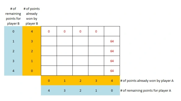Let and . The key to solving the problem of points is to look at an extended play of points.

Here’s the great insight that came from Pascal and Fermat. They looked forward and not backward. They did not base the solution on the number of points that are already won. Instead, they focused on an extended series of points to determine the share of the winning. This additional play of points is “fictitious” but it helps clarify the process. In essence, they turned the original problem of points into a problem about this additional play of points.

The original problem is: what is the fair share for player A when the game is stopped prematurely with player A having won points and player B having won points? The equivalent problem is: what is the probability of player A winning at least points of the next points where and (assuming the game has not stopped). Let’s call this probability . Let’s examine the setting of this probability. Each point is like a Bernoulli trial – either a success (player A winning it) or a failure (player B winning it). There are trials. The probability of success is in each trial. We wish to find the probability that are at least successes. What is being described is a binomial distribution. The probability being sought is:

where , and that is the number of points won by player A and is the number of points won by player B at the time the game is terminated.

The probability is the probability of player A winning the game if the game were to continue at the point of termination. This probability is the proportion of the stakes that would be awarded to player A. Of course, the proportion that should be awarded to player B would be . The quantity can be obtained from the given parameters and by using any software that has a function for the binomial distribution.

The problem of points seems to have an easy solution since the answer is so accessible. Any one who understands the binomial distribution can comprehend. It is also easy to compute probabilities for a binomial distribution using calculator or software. One thing to keep in mind is that the solution looks accessible now because of the tools and concepts that came from trails blazed by Pascal and Fermat (and because of the computing tools that we have). Tools and concepts such as Pascal’s triangle and binomial distribution were unknown to people at the time of Pascal and Fermat.

___________________________________________________________________________

Working Backward

For us, the calculation in is easily done using calculator or software. Pascal did not calculate directly and instead perform the calculation backward by using the following formula.

The formula can be derived mathematically. But doing that is not necessary. The quantity is the probability that player A will win points before player B winning points. We can derive the above formula by conditioning on the outcome of the first point. The quantity is calculated in Example 1 and Example 2. It is the average of two similar probabilities with smaller parameters.

Based on the recursive formula in , Pascal built up the answer backward, similar to the way a computer program is written. In fact, this recursive approach allows us to solve not just for one scenario, but for all the scenarios in a game of points.

Example 4
We now revisit the problem in Examples 1 and 2. Recall that the game is to play for 4 points, i.e. the first player winning 4 points collects the entire stakes of 64 (32 is contributed by each player). Each player earns a point with probability 0.5. We now show how to divide the stakes when the game is stopped at every possible stopping point.

The following diagram (Figure 1) shows the table for the share awarded to player A. The table is empty except for the top row and rightmost column (the numbers in red). The number 64 shown in the last column would be the amount awarded to player A because player A has won 4 points. The number 0 in the top means that player B has won 4 games. So player A gets nothing. Note that the bottom row highlighted in orange shows the numbers of points that have been won player A. The bottom row highlighted in blue shows the remaining points that player A needs to win in order to win the entire stakes (these are the fictitious points). Similarly, the columns highlighted in orange and blue on the left show the same information for player B.

Figure 1 – The share of the stakes awarded to player A

Now, we can use the recursive formula in to fill the table. Basically each cell is the average of the number above it and the number to the right. The parameter in is a number in the blue row. The parameter in is a number in the blue column. The following shows the results.

Figure 2 – The share of the stakes awarded to player A

For example, when player A has won 2 points and player B has won 1 point, the share for player A is 44 (the average of 32 and 56), the same answer as in Example 1 and Example 2. When player A has won 2 points and player B as won 2 points, both players are in equally competitive positions. Then each player gets 32. When player A has won 2 points and player B as won 3 points, the share for player A is 16 (the average of 0 and 32).

Essentially the formula in is the idea of using smaller steps rather than the entire extended play of points. This idea of smaller steps was preferred by Pascal. At the point where player A needs more points to win and player B needs more points to win, the idea is to play one more point. Suppose that the players know the awards to the two players after one more round. Then they should split the difference between the future awards. The calculation should begin at the point where each player only needs one more point to win (the cell with 32 in Figure 2). In that cell, we know the awards after one additional round. Taking the average of 0 and 64 gives 32. From that cell, we move down and move left on the table. Keep repeating the process until the entire table is filled in.

There is a way to tweak the table approach to work for unequal winning probability of a point. Let’s say the probability of player A winning a point is 0.6. Then the probability of player B winning a point is 0.4. The value of a given cell in the table would be the weighted average of the cell on the right (0.6 weight) with the cell above it (0.4 weight). When we know the results from playing one more round, we assign 0.6 to the result of player A winning and 0.4 to the result of player B winning. The following table shows the results.

Figure 3 – The share of the stakes awarded to player A (with 0.6 weight)

The direct formula or the table approach using the recursive formula can be easily programmed in a computer. For Pascal, the table approach is a very attractive option since the calculation can be built up from lower parameter values. In the above configuration, simply fill in the right column (the entire stakes going to player A) and the top row (player A getting nothing). Then the remaining cells are obtained by weighted average as described in formula .

We present one more example.

Example 5
Suppose that player B is a casino and player A is a visitor at the casino playing for 12 points. The house edge is 2% so that the probability of player A winning a round is 0.48. If player A desires to leave after player A has won 9 points and the house has won 6 points, what is the proportion of the stakes that should be awarded to player A?

Playing for 12 points, player A needs 3 more points to win and the house needs 6 more points to win. So we need to analyze an extended play of 3 + 6 – 1 = 8 points. For player A to win the extended play, he needs to win at least 3 points.

The answer can be obtained by computing each term in the sum (from to ). Another way is to use the BINOMDIST function in Excel as follows:

= 1-BINOMDIST(2, 8, 0.48, TRUE) = 1-0.172368083 = 0.827631917

Based on the fair division method discussed in this blog post, player A deserves 82.76% of the stakes.

___________________________________________________________________________

Remarks

In their correspondence, Pascal and Fermat came up with convincing and consistent solution to the problem of points. The earlier solutions to the problem of points were not satisfactory (to all concerned) and are sometimes inconsistent. Division of stakes only basing on the numbers points that have been won may produce extreme results. For example, if player A has won 1 point and player B has won no points, then player A would get the entire stakes. For the game described in Figure 2, for the same scenario, player A gets 42 out of 64 (42 / 64 = 0.65625), which is far from 100%.

For more detailed information on the history of the problem of points, see “A History of Mathematics” by Victor J. Katz.

___________________________________________________________________________

When a gambler asked a mathematician for help

When a gambler consistently loses large sum of money, what can he or she do? When one particular gambler, Chevalier de Méré (1607-1684), was losing a big fortune, he called a “mathematical help line”. In fact, his correspondence with Blaise Pascal (1623-1662) earned him a place in the history book. The problems that were presented by de Méré, jointly worked on by Pascal and Pierre de Fermat (1601-1665), are regarded as the beginning of the emerging academic field of probability. Chevalier de Méré was in need of help for two problems – the problem of points and on the dice problem that now bears his name. In this post we discuss the dice problem. The problem of points is discussed in the next post.

___________________________________________________________________________

The Dice Problem

There were two dice problems from Chevalier de Méré. The first game involves four rolls of a fair die. In this game, de Méré made bet with even odds on rolling at least one six when a fair die is rolled four times. His reasoning was that since getting a six in one roll of a die is (correct), the chance of getting a six in four rolls of a die would be (incorrect). With the favorable odds of 67% of winning, he reasoned that betting with even odds would be a profitable proposition. Though his calculation was incorrect, he made considerable amount of money over many years playing this game.

The second game involves twenty four rolls of a pair of fair dice. The success in the first game emboldened de Méré to make even bet on rolling one or more double sixes in twenty four rolls of a pair of dice. His reasoning was that the chance for getting a double six in one roll of a pair of dice is (correct). Then the chance of getting a double six in twenty four rolls of a pair of dice would be (incorrect). He again reasoned that betting with even odds would be profitable too.

But experience showed otherwise. As he lost a lot of money, he realized something was not quite right with the second game. In 1654, he challenged his renowned friend Blaise Pascal to find an explanation. The solution emerged in a series of letters between Pascal and Fermat. Out of this joint effort, a foundation was laid for the idea of probability as an academic subject. One particular idea that emerged was the Pascal triangle. Another one was the binomial distribution. In fact, anyone who understand the binomial distribution can very quickly see the faulty reasoning of de Méré.

___________________________________________________________________________

The Simulation

Before we get to the calculation, let’s simulate the games played by de Méré. Using random numbers generated from using the Rand() function in Excel, we simulated 100,000 iterations of each of the games. In our 100,000 simulations of the first game – rolling a die four times, there are 51,380 iterations with at least one six. This suggests that de Méré’s position would win more than half of the time, though not the odds that he believed. But it was profitable for him nonetheless.

In our 100,000 simulations of the second game – rolling a pair of dice 24 times, there are only 49,211 iterations with at least one double six. This seems to support that de Méré’s position is a losing proposition, that he would be losing his bets more than half the time.

Of course, de Méré could have done similar simulation, though in a much smaller scale, by rolling the dice himself (say, 100 times). He could have seen the light much sooner.

___________________________________________________________________________

The Calculation

Let’s see why the first game was profitable for de Méré and why the second game was not.

The First Game
In a roll of a die, there are six possible outcomes: 1, 2, 3, 4, 5, 6. If the die is fair, the probability of getting a six is . Likewise, the probability of getting no six in one roll of a fair die is .

The probability of getting no six in four rolls is:

.

Thus in four rolls of a fair die, the probability of getting at least one six is:

Thus the probability of getting at least one six in four rolls of a fair die is 0.517747. Out of 100 games, de Méré would on average win 52 games. Out of 1000 games, he would on average win 518 games. Suppose each bet is one French franc. Then de Méré would gain 36 francs for each 1000 francs in wagered. Thus he had the house’s edge of about 3.6%.

The Second Game
In a roll of a pair of dice, there are a total of 36 possible outcomes (i.e. the six outcomes of the first die combined with the six outcomes of the second die). Out of these 36 outcomes, only one of them is a double six. So, the probability of getting a double six is in rolling a pair of dice. Likewise, the probability of not getting a double six is .

The probability of getting no double six in 24 rolls of a pair of dice is:

Thus the probability of getting at least one double six in 24 rolls is:

Thus the probability of getting at least one double six in 24 rolls of a pair of fair dice is 0.4914. On average, de Méré would only win about 49 games out of 100 and his opposing side would win about 51 games out of 100 games. Out of 1000 games, he would on average win 491 games (the opposing side would win on average 509 games). With each bet as one franc, the opposing side of de Méré would win 18 francs for each 1000 francs wagered (thus the opposing side having the house’s edge of about 1.8%).

The odds indicated by the simulations discussed above are in line with the calculated results. It would be interesting to known what action did de Méré take after learning the answers. Maybe he stopped playing the second game and only played the first game. Maybe he modified the second game so that the odds of winning for him was at least even (or better).

___________________________________________________________________________