
This post discusses the coupon collector problem, a classical problem in probability.
___________________________________________________________________________
The Coupon Collector Problem
The problem is usually stated as a coupon collector trying to collect the entire set of coupons. For example, each time the coupon collector buys a product (e.g. a box of breakfast cereal), he receives a coupon, which is a prize that can be a toy or a baseball card or other interesting item. Suppose that there are 
A simplified discussion of the coupon collector problem is found in another blog post. This post is more detailed discussion.
This blog post in another blog discusses the coupon collector problem from a simulation perspective.
As shown below, if there are 5 different coupons, it takes 12 purchases on average to get all coupons. If there are 10 different types of coupons, on average it would take 30 purchases. If there are 50 different types of coupons, it would take on average 225 purchases collect the entire set. The first few coupons are obtained fairly quickly. As more and more coupons are accumulated, it is harder to get the remaining coupons. For example, for the 50-coupon case, after the 49 coupons are obtained, it takes on average 50 purchases to get the last coupon.
Suppose that the coupon collector does not want to collect the entire set and only wishes to collect 

We first consider the main case that the coupon collector wishes to collect the entire set. The problem can be cast as a random sampling from the population 


Another interpretation of the problem is that it can be viewed as an occupancy problem, which involves throwing balls into
Regardless of the interpretation, the goal is obtain information on the random variable
___________________________________________________________________________
Mean and Variance
The mean and variance of

where 


Note that each 

![\displaystyle E[C_i]=\frac{1}{p}=\frac{n}{n-(i-1)}](https://s0.wp.com/latex.php?latex=%5Cdisplaystyle+E%5BC_i%5D%3D%5Cfrac%7B1%7D%7Bp%7D%3D%5Cfrac%7Bn%7D%7Bn-%28i-1%29%7D&bg=ffffff&fg=333333&s=0&c=20201002)
![\displaystyle Var[C_i]=\frac{1-p}{p^2}=\frac{n(i-1)}{[n-(i-1)]^2}](https://s0.wp.com/latex.php?latex=%5Cdisplaystyle+Var%5BC_i%5D%3D%5Cfrac%7B1-p%7D%7Bp%5E2%7D%3D%5Cfrac%7Bn%28i-1%29%7D%7B%5Bn-%28i-1%29%5D%5E2%7D&bg=ffffff&fg=333333&s=0&c=20201002)
where 
![\displaystyle E[X_n]=\sum \limits_{i=1}^n E[C_i]=\sum \limits_{i=1}^n \frac{n}{n-(i-1)} \ \ \ \ \ \ \ \ \ \ \ \ \ \ \ \ \ \ \ \ \ \ \ \ \ \ \ \ \ \ \ \ \ \ \ \ \ (1)](https://s0.wp.com/latex.php?latex=%5Cdisplaystyle+E%5BX_n%5D%3D%5Csum+%5Climits_%7Bi%3D1%7D%5En+E%5BC_i%5D%3D%5Csum+%5Climits_%7Bi%3D1%7D%5En+%5Cfrac%7Bn%7D%7Bn-%28i-1%29%7D+%5C+%5C+%5C+%5C+%5C+%5C+%5C+%5C+%5C+%5C+%5C+%5C+%5C+%5C+%5C+%5C+%5C+%5C+%5C+%5C+%5C+%5C+%5C+%5C+%5C+%5C+%5C+%5C+%5C+%5C+%5C+%5C+%5C+%5C+%5C+%5C+%5C+%281%29&bg=ffffff&fg=333333&s=0&c=20201002)
![\displaystyle Var[X_n]=\sum \limits_{i=1}^n Var[C_i]=\sum \limits_{i=1}^n \frac{n(i-1)}{[n-(i-1)]^2} \ \ \ \ \ \ \ \ \ \ \ \ \ \ \ \ \ \ \ \ \ \ \ \ \ \ \ \ (2)](https://s0.wp.com/latex.php?latex=%5Cdisplaystyle+Var%5BX_n%5D%3D%5Csum+%5Climits_%7Bi%3D1%7D%5En+Var%5BC_i%5D%3D%5Csum+%5Climits_%7Bi%3D1%7D%5En+%5Cfrac%7Bn%28i-1%29%7D%7B%5Bn-%28i-1%29%5D%5E2%7D+%5C+%5C+%5C+%5C+%5C+%5C+%5C+%5C+%5C+%5C+%5C+%5C+%5C+%5C+%5C+%5C+%5C+%5C+%5C+%5C+%5C+%5C+%5C+%5C+%5C+%5C+%5C+%5C+%282%29&bg=ffffff&fg=333333&s=0&c=20201002)
The expectation ![E[X_n]](https://s0.wp.com/latex.php?latex=E%5BX_n%5D&bg=ffffff&fg=333333&s=0&c=20201002)
![\displaystyle E[X_n]=n \ \biggl[\frac{1}{n}+ \cdots + \frac{1}{3}+ \frac{1}{2} + 1\biggr]=n \ H_n \ \ \ \ \ \ \ \ \ \ \ \ \ \ \ \ \ \ \ \ \ \ \ \ \ \ \ \ \ (3)](https://s0.wp.com/latex.php?latex=%5Cdisplaystyle+E%5BX_n%5D%3Dn+%5C+%5Cbiggl%5B%5Cfrac%7B1%7D%7Bn%7D%2B+%5Ccdots+%2B+%5Cfrac%7B1%7D%7B3%7D%2B+%5Cfrac%7B1%7D%7B2%7D+%2B+1%5Cbiggr%5D%3Dn+%5C+H_n++%5C+%5C+%5C+%5C+%5C+%5C+%5C+%5C+%5C+%5C+%5C+%5C+%5C+%5C+%5C+%5C+%5C+%5C+%5C+%5C+%5C+%5C+%5C+%5C+%5C+%5C+%5C+%5C+%5C+%283%29&bg=ffffff&fg=333333&s=0&c=20201002)
The quantity 


![E[X_n] \rightarrow \infty](https://s0.wp.com/latex.php?latex=E%5BX_n%5D+%5Crightarrow+%5Cinfty&bg=ffffff&fg=333333&s=0&c=20201002)
Table 1
![\begin{array}{cccccc} \text{Number of} & \text{ } & \text{Expected Number of Trials} & \text{ } & \text{Expected Total Number} & \\ \text{Coupons} & \text{ } & \text{per Coupon} & \text{ } & \text{of Trials (rounded up)} & \\ n & \text{ } & E[H_n] & \text{ } & E[X_n] & \\ \text{ } & \text{ } & \text{ } & \text{ } & \text{ } & \\ 1 & \text{ } & 1.0000 & & 1 & \\ 2 & \text{ } & 1.5000 & & 3 & \\ 3 & \text{ } & 1.8333 & & 6 & \\ 4 & \text{ } & 2.0833 & & 9 & \\ 5 & \text{ } & 2.2833 & & 12 & \\ 6 & \text{ } & 2.4500 & & 15 & \\ 7 & \text{ } & 2.5929 & & 19 & \\ 8 & \text{ } & 2.7179 & & 22 & \\ 9 & \text{ } & 2.8290 & & 26 & \\ 10 & \text{ } & 2.9290 & & 30 & \\ 20 & \text{ } & 3.5977 & & 72 & \\ 30 & \text{ } & 3.9950 & & 120 & \\ 40 & \text{ } & 4.2785 & & 172 & \\ 50 & \text{ } & 4.4992 & & 225 & \\ 60 & \text{ } & 4.6799 & & 281 & \\ 70 & \text{ } & 4.8328 & & 339 & \\ 80 & \text{ } & 4.9655 & & 398 & \\ 90 & \text{ } & 5.0826 & & 458 & \\ 100 & \text{ } & 5.1874 & & 519 & \\ \end{array}](https://s0.wp.com/latex.php?latex=%5Cbegin%7Barray%7D%7Bcccccc%7D++++%5Ctext%7BNumber+of%7D+%26++%5Ctext%7B+%7D+%26+%5Ctext%7BExpected+Number+of+Trials%7D++%26+%5Ctext%7B+%7D+%26+%5Ctext%7BExpected+Total+Number%7D+%26++%5C%5C++%5Ctext%7BCoupons%7D+%26++%5Ctext%7B+%7D+%26+%5Ctext%7Bper+Coupon%7D++%26+%5Ctext%7B+%7D+%26+%5Ctext%7Bof+Trials+%28rounded+up%29%7D+%26++%5C%5C++++n+%26++%5Ctext%7B+%7D+%26+E%5BH_n%5D++%26+%5Ctext%7B+%7D+%26+E%5BX_n%5D+%26++%5C%5C++%5Ctext%7B+%7D+%26+++%5Ctext%7B+%7D+%26+%5Ctext%7B+%7D+%26+%5Ctext%7B+%7D+%26+%5Ctext%7B+%7D+%26++%5C%5C+++1+%26+++%5Ctext%7B+%7D+%26+1.0000+%26++%26+1+%26++%5C%5C+++2+%26+++%5Ctext%7B+%7D+%26+1.5000+%26++%26+3+%26++%5C%5C+++3+%26+++%5Ctext%7B+%7D+%26+1.8333+%26++%26+6+%26++%5C%5C+++4+%26+++%5Ctext%7B+%7D+%26+2.0833+%26++%26+9+%26++%5C%5C+++5+%26+++%5Ctext%7B+%7D+%26+2.2833+%26++%26+12+%26++%5C%5C+++6+%26+++%5Ctext%7B+%7D+%26+2.4500+%26++%26+15+%26++%5C%5C+++7+%26+++%5Ctext%7B+%7D+%26+2.5929+%26++%26+19+%26++%5C%5C+++8+%26+++%5Ctext%7B+%7D+%26+2.7179+%26++%26+22+%26++%5C%5C+++++++++9+%26+++%5Ctext%7B+%7D+%26+2.8290+%26++%26+26+%26++%5C%5C+++10+%26+++%5Ctext%7B+%7D+%26+2.9290+%26++%26+30+%26++%5C%5C+++20+%26+++%5Ctext%7B+%7D+%26+3.5977+%26++%26+72+%26++%5C%5C+++30+%26+++%5Ctext%7B+%7D+%26+3.9950+%26++%26+120+%26++%5C%5C+++40+%26+++%5Ctext%7B+%7D+%26+4.2785+%26++%26+172+%26++%5C%5C+++50+%26+++%5Ctext%7B+%7D+%26+4.4992+%26++%26+225+%26++%5C%5C++++60+%26++%5Ctext%7B+%7D+%26+4.6799+%26++%26+281+%26++%5C%5C++++70+%26++%5Ctext%7B+%7D+%26+4.8328+%26++%26+339+%26++%5C%5C++80+%26++%5Ctext%7B+%7D+%26+4.9655+%26++%26+398+%26++%5C%5C++90+%26++%5Ctext%7B+%7D+%26+5.0826+%26++%26+458+%26++%5C%5C++100+%26++%5Ctext%7B+%7D+%26+5.1874+%26++%26+519+%26++%5C%5C++++%5Cend%7Barray%7D&bg=ffffff&fg=333333&s=0&c=20201002)
Table 1 gives an estimate on how long to expect to collect the entire set of coupons for selected coupon sizes. The third column gives the expected total number of purchases to obtain the entire coupon set. The second column gives an estimate of how many purchases on average to obtain one coupon. For the 50-coupon case, it takes on average about 4.5 purchases to obtain one coupon. However, it does not tell the whole story. To get the 50th coupon, it takes on average 50 trials. Note that ![E[C_{50}]=50](https://s0.wp.com/latex.php?latex=E%5BC_%7B50%7D%5D%3D50&bg=ffffff&fg=333333&s=0&c=20201002)
___________________________________________________________________________
The Occupancy Problem
We now view the coupon collector problem as an occupancy problem in order to leverage a formula from a previous post. Suppose that we randomly throw 


where 
The notation 


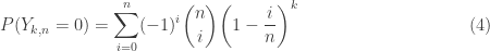
The formula (5) gives the probability of having 
![P[Y_{k,n}=n-w]](https://s0.wp.com/latex.php?latex=P%5BY_%7Bk%2Cn%7D%3Dn-w%5D&bg=ffffff&fg=333333&s=0&c=20201002)
___________________________________________________________________________
The Probability Function
We now discuss the probability function of the random variable ![P[X_n=k]](https://s0.wp.com/latex.php?latex=P%5BX_n%3Dk%5D&bg=ffffff&fg=333333&s=0&c=20201002)


![P(X_n=k]=P[Y_{k,n}=0 \text{ and } Y_{k-1,n}=1] \ \ \ \ \ \ \ \ \ \ \ \ \ \ \ \ \ \ \ \ \ \ \ \ \ \ \ (6)](https://s0.wp.com/latex.php?latex=P%28X_n%3Dk%5D%3DP%5BY_%7Bk%2Cn%7D%3D0+%5Ctext%7B+and+%7D+Y_%7Bk-1%2Cn%7D%3D1%5D++%5C+%5C+%5C+%5C+%5C+%5C+%5C+%5C+%5C+%5C+%5C+%5C+%5C+%5C+%5C+%5C+%5C+%5C+%5C+%5C+%5C+%5C+%5C+%5C+%5C+%5C+%5C+%286%29&bg=ffffff&fg=333333&s=0&c=20201002)
Consider the following derivation.
![\displaystyle \begin{aligned} P(X_n=k]&=P[Y_{k,n}=0 \text{ and } Y_{k-1,n}=1] \\&=P[Y_{k,n}=0 \ \lvert \ Y_{k-1,n}=1] \times P[Y_{k-1,n}=1] \\&=\frac{1}{n} \times \binom{n}{1} \sum \limits_{i=0}^{n-1} (-1)^i \binom{n-1}{i} \biggl[ 1-\frac{1+i}{n} \biggr]^{k-1} \\&=\sum \limits_{i=0}^{n-1} (-1)^i \binom{n-1}{i} \biggl[ 1-\frac{1+i}{n} \biggr]^{k-1} \ \ \ \ \ \ \ \ \ \ \ \ \ \ \ \ \ \ \ \ (7) \end{aligned}](https://s0.wp.com/latex.php?latex=%5Cdisplaystyle+%5Cbegin%7Baligned%7D+P%28X_n%3Dk%5D%26%3DP%5BY_%7Bk%2Cn%7D%3D0+%5Ctext%7B+and+%7D+Y_%7Bk-1%2Cn%7D%3D1%5D+%5C%5C%26%3DP%5BY_%7Bk%2Cn%7D%3D0+%5C+%5Clvert+%5C+Y_%7Bk-1%2Cn%7D%3D1%5D+%5Ctimes+P%5BY_%7Bk-1%2Cn%7D%3D1%5D+%5C%5C%26%3D%5Cfrac%7B1%7D%7Bn%7D+%5Ctimes+%5Cbinom%7Bn%7D%7B1%7D+%5Csum+%5Climits_%7Bi%3D0%7D%5E%7Bn-1%7D+%28-1%29%5Ei+%5Cbinom%7Bn-1%7D%7Bi%7D+%5Cbiggl%5B+1-%5Cfrac%7B1%2Bi%7D%7Bn%7D+%5Cbiggr%5D%5E%7Bk-1%7D+%5C%5C%26%3D%5Csum+%5Climits_%7Bi%3D0%7D%5E%7Bn-1%7D+%28-1%29%5Ei+%5Cbinom%7Bn-1%7D%7Bi%7D+%5Cbiggl%5B+1-%5Cfrac%7B1%2Bi%7D%7Bn%7D+%5Cbiggr%5D%5E%7Bk-1%7D+%5C+%5C+%5C+%5C+%5C+%5C+%5C+%5C+%5C+%5C+%5C+%5C+%5C+%5C+%5C+%5C+%5C+%5C+%5C+%5C+%287%29+%5Cend%7Baligned%7D&bg=ffffff&fg=333333&s=0&c=20201002)
where
Rather than memorizing the probability function in (7), a better way is to focus on the thought process that is inherent in (6).
One comment about the calculation for (7). The summation for
![P[X_6>15]=1-P[6 \le X_6 \le 14]](https://s0.wp.com/latex.php?latex=P%5BX_6%3E15%5D%3D1-P%5B6+%5Cle+X_6+%5Cle+14%5D&bg=ffffff&fg=333333&s=0&c=20201002) .
.
Unless the number of values for
___________________________________________________________________________
Examples
Example 1
Suppose that a fair die is rolled until all 6 faces have appeared. Find the mean number of rolls and the variance of the number of rolls. What is the probability that it will take at least 12 rolls? What is the probability that it will take more than 15 rolls?
Using the notation developed above, the random variable of interest is 
![\displaystyle E[X_6]=6 \ \biggl[ 1 + \frac{1}{2}+\frac{1}{3}+\frac{1}{4}+\frac{1}{5}+\frac{1}{6} \biggr]=6 \times 2.45 = 14.7 \approx 15](https://s0.wp.com/latex.php?latex=%5Cdisplaystyle+E%5BX_6%5D%3D6+%5C+%5Cbiggl%5B+1+%2B+%5Cfrac%7B1%7D%7B2%7D%2B%5Cfrac%7B1%7D%7B3%7D%2B%5Cfrac%7B1%7D%7B4%7D%2B%5Cfrac%7B1%7D%7B5%7D%2B%5Cfrac%7B1%7D%7B6%7D+%5Cbiggr%5D%3D6+%5Ctimes+2.45+%3D+14.7+%5Capprox+15&bg=ffffff&fg=333333&s=0&c=20201002)
![\displaystyle Var[X_6]=\sum \limits_{i=1}^6 \frac{6(i-1)}{[6-(i-1)]^2}=38.99](https://s0.wp.com/latex.php?latex=%5Cdisplaystyle+Var%5BX_6%5D%3D%5Csum+%5Climits_%7Bi%3D1%7D%5E6+%5Cfrac%7B6%28i-1%29%7D%7B%5B6-%28i-1%29%5D%5E2%7D%3D38.99&bg=ffffff&fg=333333&s=0&c=20201002)
The following is the probability function for
![\displaystyle P[X_6=k]=\sum \limits_{i=0}^{5} (-1)^i \binom{5}{i} \biggl[ 1-\frac{1+i}{6} \biggr]^{k-1}](https://s0.wp.com/latex.php?latex=%5Cdisplaystyle+P%5BX_6%3Dk%5D%3D%5Csum+%5Climits_%7Bi%3D0%7D%5E%7B5%7D+%28-1%29%5Ei+%5Cbinom%7B5%7D%7Bi%7D+%5Cbiggl%5B+1-%5Cfrac%7B1%2Bi%7D%7B6%7D+%5Cbiggr%5D%5E%7Bk-1%7D&bg=ffffff&fg=333333&s=0&c=20201002)
where

For each ![P[X_6=k]](https://s0.wp.com/latex.php?latex=P%5BX_6%3Dk%5D&bg=ffffff&fg=333333&s=0&c=20201002)
![P[X_6 \ge 12]=1-P[6 \le X_6 \le 11]=1-0.356206419=0.643793581](https://s0.wp.com/latex.php?latex=P%5BX_6+%5Cge+12%5D%3D1-P%5B6+%5Cle+X_6+%5Cle+11%5D%3D1-0.356206419%3D0.643793581&bg=ffffff&fg=333333&s=0&c=20201002)
![P[X_6 > 15]=1-P[6 \le X_6 \le 15]=1-0.644212739=0.355787261](https://s0.wp.com/latex.php?latex=P%5BX_6+%3E+15%5D%3D1-P%5B6+%5Cle+X_6+%5Cle+15%5D%3D1-0.644212739%3D0.355787261&bg=ffffff&fg=333333&s=0&c=20201002)
Even though the average number of trials is 15, there is still a significant probability that it will take more than 15 trials. This is because the variance is quite large.

Example 2
An Internet startup is rapidly hiring new employees. What is the expected number of new employees until all birth months are represented? Assume that the 12 birth months are equally likely. What is the probability that the company will have to hire more than 25 employees? If the company currently has more than 25 employees with less than 12 birth months, what is the probability that it will have to hire more than 35 employees to have all 12 birth months represented in the company?
The random variable of interest is 
![\displaystyle E[X_{12}]=12 \ \biggl[ 1 + \frac{1}{2}+\frac{1}{3}+\cdots +\frac{1}{12} \biggr]=37.23852814 \approx 38](https://s0.wp.com/latex.php?latex=%5Cdisplaystyle+E%5BX_%7B12%7D%5D%3D12+%5C+%5Cbiggl%5B+1+%2B+%5Cfrac%7B1%7D%7B2%7D%2B%5Cfrac%7B1%7D%7B3%7D%2B%5Ccdots+%2B%5Cfrac%7B1%7D%7B12%7D+%5Cbiggr%5D%3D37.23852814+%5Capprox+38&bg=ffffff&fg=333333&s=0&c=20201002)
![\displaystyle P[X_{12}=k]=\sum \limits_{i=0}^{11} (-1)^i \binom{11}{i} \biggl[ 1-\frac{1+i}{12} \biggr]^{k-1}](https://s0.wp.com/latex.php?latex=%5Cdisplaystyle+P%5BX_%7B12%7D%3Dk%5D%3D%5Csum+%5Climits_%7Bi%3D0%7D%5E%7B11%7D+%28-1%29%5Ei+%5Cbinom%7B11%7D%7Bi%7D+%5Cbiggl%5B+1-%5Cfrac%7B1%2Bi%7D%7B12%7D+%5Cbiggr%5D%5E%7Bk-1%7D&bg=ffffff&fg=333333&s=0&c=20201002)
where

Performing the calculation in Excel, we obtain the following probabilities.
![P[X_{12} > 25]=1-P[12 \le X_{12} \le 25]=1-0.181898592=0.818101408](https://s0.wp.com/latex.php?latex=P%5BX_%7B12%7D+%3E+25%5D%3D1-P%5B12+%5Cle+X_%7B12%7D+%5Cle+25%5D%3D1-0.181898592%3D0.818101408&bg=ffffff&fg=333333&s=0&c=20201002)
![P[X_{12} > 35]=1-P[12 \le X_{12} \le 35]=1-0.531821149=0.468178851](https://s0.wp.com/latex.php?latex=P%5BX_%7B12%7D+%3E+35%5D%3D1-P%5B12+%5Cle+X_%7B12%7D+%5Cle+35%5D%3D1-0.531821149%3D0.468178851&bg=ffffff&fg=333333&s=0&c=20201002)
![\displaystyle P[X_{12} > 35 \ \lvert \ X_{12} > 25]=\frac{P[X_{12} > 35]}{P[X_{12} > 25]}=\frac{0.468178851}{0.818101408}=0.572274838](https://s0.wp.com/latex.php?latex=%5Cdisplaystyle+P%5BX_%7B12%7D+%3E+35+%5C+%5Clvert+%5C+X_%7B12%7D+%3E+25%5D%3D%5Cfrac%7BP%5BX_%7B12%7D+%3E+35%5D%7D%7BP%5BX_%7B12%7D+%3E+25%5D%7D%3D%5Cfrac%7B0.468178851%7D%7B0.818101408%7D%3D0.572274838&bg=ffffff&fg=333333&s=0&c=20201002)
___________________________________________________________________________
A Special Case
We now consider the special case that the coupon collector only wishes to collect 

where
Thus ![E[X_{n,r}]](https://s0.wp.com/latex.php?latex=E%5BX_%7Bn%2Cr%7D%5D&bg=ffffff&fg=333333&s=0&c=20201002)
![Var[X_{n,r}]](https://s0.wp.com/latex.php?latex=Var%5BX_%7Bn%2Cr%7D%5D&bg=ffffff&fg=333333&s=0&c=20201002)
For the probability function of 


![P[X_{n,r}=k]=P[Y_{k,n}=n-r \text{ and } Y_{k-1,n}=n-r+1] \ \ \ \ \ \ \ \ \ \ \ \ \ \ \ \ \ (9)](https://s0.wp.com/latex.php?latex=P%5BX_%7Bn%2Cr%7D%3Dk%5D%3DP%5BY_%7Bk%2Cn%7D%3Dn-r+%5Ctext%7B+and+%7D+Y_%7Bk-1%2Cn%7D%3Dn-r%2B1%5D++%5C+%5C+%5C+%5C+%5C+%5C+%5C+%5C+%5C+%5C+%5C+%5C+%5C+%5C+%5C+%5C+%5C+%289%29&bg=ffffff&fg=333333&s=0&c=20201002)
Here’s the important components that need to go into ![P[X_{n,r}=k]](https://s0.wp.com/latex.php?latex=P%5BX_%7Bn%2Cr%7D%3Dk%5D&bg=ffffff&fg=333333&s=0&c=20201002)
![\displaystyle P[Y_{k-1,n}=n-r+1]=\binom{n}{n-r+1} \sum \limits_{i=0}^{r-1} (-1)^i \binom{r-1}{i} \biggl[ 1-\frac{n-r+1+i}{n} \biggr]^{k-1}](https://s0.wp.com/latex.php?latex=%5Cdisplaystyle+P%5BY_%7Bk-1%2Cn%7D%3Dn-r%2B1%5D%3D%5Cbinom%7Bn%7D%7Bn-r%2B1%7D+%5Csum+%5Climits_%7Bi%3D0%7D%5E%7Br-1%7D+%28-1%29%5Ei+%5Cbinom%7Br-1%7D%7Bi%7D+%5Cbiggl%5B+1-%5Cfrac%7Bn-r%2B1%2Bi%7D%7Bn%7D+%5Cbiggr%5D%5E%7Bk-1%7D&bg=ffffff&fg=333333&s=0&c=20201002)
![\displaystyle P[Y_{k,n}=n-r \ \lvert \ Y_{k-1,n}=n-r+1]=\frac{n-r+1}{n}](https://s0.wp.com/latex.php?latex=%5Cdisplaystyle+P%5BY_%7Bk%2Cn%7D%3Dn-r+%5C+%5Clvert+%5C+Y_%7Bk-1%2Cn%7D%3Dn-r%2B1%5D%3D%5Cfrac%7Bn-r%2B1%7D%7Bn%7D&bg=ffffff&fg=333333&s=0&c=20201002)
Multiply the above two probabilities together produces the desired probability 
![\displaystyle P[X_{n,r}=k]=\binom{n-1}{r-1} \sum \limits_{i=0}^{r-1} (-1)^i \binom{r-1}{i} \biggl[ 1-\frac{n-r+1+i}{n} \biggr]^{k-1} \ \ \ \ \ \ \ \ (10)](https://s0.wp.com/latex.php?latex=%5Cdisplaystyle+P%5BX_%7Bn%2Cr%7D%3Dk%5D%3D%5Cbinom%7Bn-1%7D%7Br-1%7D+%5Csum+%5Climits_%7Bi%3D0%7D%5E%7Br-1%7D+%28-1%29%5Ei+%5Cbinom%7Br-1%7D%7Bi%7D+%5Cbiggl%5B+1-%5Cfrac%7Bn-r%2B1%2Bi%7D%7Bn%7D+%5Cbiggr%5D%5E%7Bk-1%7D+%5C+%5C+%5C+%5C+%5C+%5C+%5C+%5C+%2810%29&bg=ffffff&fg=333333&s=0&c=20201002)
Note that when 
Example 3
Consider the 6-coupon case discussed in Example 1. Suppose that the coupon collector is interested in collecting 
The random variable of interest is 
![\displaystyle E[X_{6,4}]=6 \biggl[ \frac{1}{6}+\frac{1}{5}+\frac{1}{4}+\frac{1}{3} \biggr]=5.7 \approx 6](https://s0.wp.com/latex.php?latex=%5Cdisplaystyle+E%5BX_%7B6%2C4%7D%5D%3D6+%5Cbiggl%5B+%5Cfrac%7B1%7D%7B6%7D%2B%5Cfrac%7B1%7D%7B5%7D%2B%5Cfrac%7B1%7D%7B4%7D%2B%5Cfrac%7B1%7D%7B3%7D+%5Cbiggr%5D%3D5.7+%5Capprox+6&bg=ffffff&fg=333333&s=0&c=20201002)
Note that it is much faster to obtain 4 coupons than the entire set of six. The following gives the probability function for
![\displaystyle P[X_{6,4}=k]=\binom{5}{3} \sum \limits_{i=0}^{3} (-1)^i \binom{3}{i} \biggl[ 1-\frac{3+i}{6} \biggr]^{k-1}](https://s0.wp.com/latex.php?latex=%5Cdisplaystyle+P%5BX_%7B6%2C4%7D%3Dk%5D%3D%5Cbinom%7B5%7D%7B3%7D+%5Csum+%5Climits_%7Bi%3D0%7D%5E%7B3%7D+%28-1%29%5Ei+%5Cbinom%7B3%7D%7Bi%7D+%5Cbiggl%5B+1-%5Cfrac%7B3%2Bi%7D%7B6%7D+%5Cbiggr%5D%5E%7Bk-1%7D&bg=ffffff&fg=333333&s=0&c=20201002)
where 
Performing the calculations in Excel gives the following probabilities.
![P[X_{6,4} > 6]=1-P[12 \le X_{12} \le 25]=1-0.74845679=0.25154321](https://s0.wp.com/latex.php?latex=P%5BX_%7B6%2C4%7D+%3E+6%5D%3D1-P%5B12+%5Cle+X_%7B12%7D+%5Cle+25%5D%3D1-0.74845679%3D0.25154321&bg=ffffff&fg=333333&s=0&c=20201002)
![P[X_{6,4} > 8]=1-P[12 \le X_{12} \le 35]=1-0.928712277=0.071287723](https://s0.wp.com/latex.php?latex=P%5BX_%7B6%2C4%7D+%3E+8%5D%3D1-P%5B12+%5Cle+X_%7B12%7D+%5Cle+35%5D%3D1-0.928712277%3D0.071287723&bg=ffffff&fg=333333&s=0&c=20201002)
The first probability shows there is still a good chance that it will take more then the mean number of trials to get 4 coupons. The wait time is much less than in Example 1 since the probability of wait time more than 8 is fairly small.
___________________________________________________________________________
Moment Generating Function
One distributional quantity that is easy to obtain is the moment generating function (MGF) for the random variable
![\displaystyle M_{X_n}(t)=\prod \limits_{i=1}^n \frac{[n-(i-1)] e^t}{n-(i-1) e^t} \ \ \ \ \ \ \ \ \ \ \ \ \ \ \ \ \ \ \ \ \ \ \ \ \ \ \ \ \ \ \ \ \ \ \ \ \ \ \ \ \ \ \ \ \ (11)](https://s0.wp.com/latex.php?latex=%5Cdisplaystyle+M_%7BX_n%7D%28t%29%3D%5Cprod+%5Climits_%7Bi%3D1%7D%5En+%5Cfrac%7B%5Bn-%28i-1%29%5D+e%5Et%7D%7Bn-%28i-1%29+e%5Et%7D+%5C+%5C+%5C+%5C+%5C+%5C+%5C+%5C+%5C+%5C+%5C+%5C+%5C+%5C+%5C+%5C+%5C+%5C+%5C+%5C+%5C+%5C+%5C+%5C+%5C+%5C+%5C+%5C+%5C+%5C+%5C+%5C+%5C+%5C+%5C+%5C+%5C+%5C+%5C+%5C+%5C+%5C+%5C+%5C+%5C+%2811%29&bg=ffffff&fg=333333&s=0&c=20201002)
![\displaystyle M_{X_{n,r}}(t)=\prod \limits_{i=1}^r \frac{[n-(i-1)] e^t}{n-(i-1) e^t} \ \ \ \ \ \ \ \ \ \ \ \ \ \ \ \ \ \ \ \ \ \ \ \ \ \ \ \ \ \ \ \ \ \ \ \ \ \ \ \ \ \ \ (12)](https://s0.wp.com/latex.php?latex=%5Cdisplaystyle+M_%7BX_%7Bn%2Cr%7D%7D%28t%29%3D%5Cprod+%5Climits_%7Bi%3D1%7D%5Er+%5Cfrac%7B%5Bn-%28i-1%29%5D+e%5Et%7D%7Bn-%28i-1%29+e%5Et%7D+%5C+%5C+%5C+%5C+%5C+%5C+%5C+%5C+%5C+%5C+%5C+%5C+%5C+%5C+%5C+%5C+%5C+%5C+%5C+%5C+%5C+%5C+%5C+%5C+%5C+%5C+%5C+%5C+%5C+%5C+%5C+%5C+%5C+%5C+%5C+%5C+%5C+%5C+%5C+%5C+%5C+%5C+%5C+%2812%29&bg=ffffff&fg=333333&s=0&c=20201002)
___________________________________________________________________________


Pingback: The coupon collector problem | All Math Considered
Pingback: Celebrate the year of the rooster | All Math Considered
Pingback: Five probability problems to help us think better | Math in the Spotlight
Pingback: First step analysis and fundamental matrix | Topics in Probability
Pingback: Probability problems using Markov chains | A Blog on Probability and Statistics
Pingback: Making use of Markov chains – Climbing Math Everest