
This is a continuation of the previous post The sign test. Examples 1 and 2 are presented in the previous post. In this post we present three more examples. Example 3 is a matched pairs problem and is an example demonstrating that the sign test may not as powerful as the t-test when the population is close to normal. Example 4 is a one-sample location problem. Example 5 is an example of an application of the sign test when the outcomes of the study or experiment are not numerical. For more information about distribution-free inferences, see [Hollander & Wolfe].
Example 3
Courses in introductory statistics are increasingly popular at community colleges across the United States. These are statistics courses that teach basic concepts of descriptive statistics, probability notions and basic inferential statistical procedures such as one and two-sample t procedures. A certain teacher of statistics at a local community college believes that taking such a course improves students’ quantitative skills. At the beginning of one semester, this professor administered a quantitative diagnostic test to a group of 15 students taking an introductory statistics course. At the end of the semester, the professor administered a second quantitative diagnostic test. The maximum possible score on each test is 50. Though the second test was at a similar level of difficulty as the first test, the questions in the second test were different and the contexts of the problems were different. Thus simply taking the first test should not improve the second test. The following matrices show the scores before and after taking the statistics course:
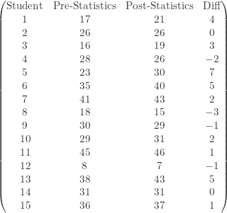
Is there evidence that taking introductory statistics course at community colleges improves students’ quantitative skills? Do the analysis using the sign test.
For a given student, let 

![p=P[X>Y]](https://s0.wp.com/latex.php?latex=p%3DP%5BX%3EY%5D&bg=ffffff&fg=333333&s=-1&c=20201002)

Another interpretation of the above alternative hypothesis is that the median of the post-statistics quantitative scores has moved upward. Let 

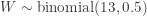

![\displaystyle \text{P-value}=P[W \ge 9]=\sum \limits_{k=9}^{13} \binom{13}{k} \biggl(\frac{1}{2}\biggr)^{13}=0.1334](https://s0.wp.com/latex.php?latex=%5Cdisplaystyle+%5Ctext%7BP-value%7D%3DP%5BW+%5Cge+9%5D%3D%5Csum+%5Climits_%7Bk%3D9%7D%5E%7B13%7D+%5Cbinom%7B13%7D%7Bk%7D+%5Cbiggl%28%5Cfrac%7B1%7D%7B2%7D%5Cbiggr%29%5E%7B13%7D%3D0.1334&bg=ffffff&fg=333333&s=-1&c=20201002)
If we want to set the probability of a type I error at 0.10, we would not reject the null hypothesis
The data set for the differences in scores appears symmetric and has no strong skewness and no obvious outliers. So it should be safe to use the t-test. With 


We obtain: t-score=2.08 and the P-value=0.028. Thus with the t-test, we would reject the null hypothesis and have the opposite conclusion. Because the sign test does not use all the available information in the data, it is not as powerful as the t-test.
Example 4
Acid rain is an environmental challenge in many places around the world. It refers to rain or any other form of precipitation that is unusually acidic, i.e. rainwater having elevated levels of hydrogen ions (low pH). The measure of pH is a measure of the acidity or basicity of a solution and has a scale ranging from 0 to 14. Distilled water, with carbon dioxide removed, has a neutral pH level of 7. Liquids with a pH less than 7 are acidic. However, even unpolluted rainwater is slightly acidic with pH varying between 5.2 to 6.0 due to the fact that carbon dioxide and water in the air react together to form carbonic acid. Thus, rainwater is only considered acidic if the pH level is less than 5.2.
In a remote region in Washington state, an enviromental biologist measured the pH levels of rainwater and obtained the following data for 16 rainwater samples on 16 different dates:
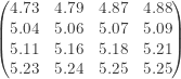
Is there reason to believe that the rainwater from this region is considered acidic (less than 5.2)? Use the sign test to perform the analysis.
Let 
![p=P[5.2>X]=P[5.2-X>0]](https://s0.wp.com/latex.php?latex=p%3DP%5B5.2%3EX%5D%3DP%5B5.2-X%3E0%5D&bg=ffffff&fg=333333&s=-1&c=20201002)

The null hypothesis
Let 
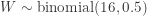

![\displaystyle \text{P-value}=P[W \ge 11]=\sum \limits_{k=11}^{16} \binom{16}{k} \biggl(\frac{1}{2}\biggr)^{16}=0.1051](https://s0.wp.com/latex.php?latex=%5Cdisplaystyle+%5Ctext%7BP-value%7D%3DP%5BW+%5Cge+11%5D%3D%5Csum+%5Climits_%7Bk%3D11%7D%5E%7B16%7D+%5Cbinom%7B16%7D%7Bk%7D+%5Cbiggl%28%5Cfrac%7B1%7D%7B2%7D%5Cbiggr%29%5E%7B16%7D%3D0.1051&bg=ffffff&fg=333333&s=-1&c=20201002)
At the level of significance 
Example 5
There are two statistics instructors who are both sought after by students in a local college. Let’s call them instructor A and instructor B. The math department conducted a survey to find out who is more popular with the students. In surveying 15 students, the department found that 11 of the students prefer instructor B over instructor A. Use the sign test to test the hypothesis of no difference in popularity against the alternative hypothesis that instructor B is more popular.
More than 
![\displaystyle \text{P-value}=P[W \ge 11]=\sum \limits_{k=11}^{15} \binom{15}{k} \biggl(\frac{1}{2}\biggr)^{15}=0.05923](https://s0.wp.com/latex.php?latex=%5Cdisplaystyle+%5Ctext%7BP-value%7D%3DP%5BW+%5Cge+11%5D%3D%5Csum+%5Climits_%7Bk%3D11%7D%5E%7B15%7D+%5Cbinom%7B15%7D%7Bk%7D+%5Cbiggl%28%5Cfrac%7B1%7D%7B2%7D%5Cbiggr%29%5E%7B15%7D%3D0.05923&bg=ffffff&fg=333333&s=-1&c=20201002)
This P-value suggests that we have strong evidence that instructor B is more popular among the students.
Reference
Myles Hollander and Douglas A. Wolfe, Non-parametric Statistical Methods, Second Edition, Wiley (1999)

Loved the Article. Clear and Simple and ideal for my studnts. Big Thumbs up
how do i enter that into my t-i
3. A group of 11 students selected at random secured the grade points: 1.5, 2.2, 0.9, 1.3, 2.0, 1.6, 1.8, 1.5, 2.0, 1.2 and 1.7 (out of 3). Use the sign test to test the hypothesis that intelligence is a random function (with a median of 1.8) at 5% level of significance
What is the a-level of example 5 ?
If a-LEVEL is 5 %
We should accept the null hypothesis..?