Calculating order statistics using multinomial probabilities

Consider a random sample $X_1,X_2,\cdots,X_n$ drawn from a continuous distribution. Rank the sample items in increasing order, resulting in a ranked sample $Y_1<Y_2<\cdots <Y_n$ where $Y_1$ is the smallest sample item, $Y_2$ is the second smallest sample item and so on. The items in the ranked sample are called the order statistics. Recently the author of this blog was calculating a conditional probability such as $P(Y_2>4 \ | \ Y_2>3)$ . One way to do this is to calculate the distribution function $P(Y_2 \le t)$ . What about the probability $P(Y_5>4 \ | \ Y_2>3)$ ? Since this one involves two order statistics, the author of this blog initially thought that calculating $P(Y_5>4 \ | \ Y_2>3)$ would require knowing the joint probability distribution of the order statistics $Y_1,Y_2,\cdots ,Y_n$ . It turns out that a joint distribution may not be needed. Instead, we can calculate a conditional probability such as $P(Y_5>4 \ | \ Y_2>3)$ using multinomial probabilities. In this post, we demonstrate how this is done using examples. Practice problems are found in here.

The calculation described here can be lengthy and tedious if the sample size is large. To make the calculation more manageable, the examples here have relatively small sample size. To keep the multinomial probabilities easier to calculate, the random samples are drawn from a uniform distribution. The calculation for larger sample sizes from other distributions is better done using a technology solution. In any case, the calculation described here is a great way to practice working with order statistics and multinomial probabilities.

________________________________________________________________________

The multinomial angle

In this post, the order statistics $Y_1<Y_2<\cdots <Y_n$ are resulted from ranking the random sample $X_1,X_2,\cdots,X_n$ , which is drawn from a continuous distribution with distribution function $F(x)=P(X \le x)$ . For the $j$ th order statistic, the calculation often begins with its distribution function $P(Y_j \le t)$ .

Here’s the thought process for calculating $P(Y_j \le t)$ . In drawing the random sample $X_1,X_2,\cdots,X_n$ , make a note of the items $\le t$ and the items $>t$ . For the event $Y_j \le t$ to happen, there must be at least $j$ many sample items $X_i$ that are $\le t$ . For the event $Y_j > t$ to happen, there can be only at most $j-1$ many sample items $X_i$ $\le t$ . So to calculate $P(Y_j \le t)$ , simply find out the probability of having $j$ or more sample items $\le t$ . To calculate $P(Y_j > t)$ , find the probability of having at most $j-1$ sample items $\le t$ .

$\displaystyle P(Y_j \le t)=\sum \limits_{k=j}^n \binom{n}{k} \ \biggl[ F(t) \biggr]^k \ \biggl[1-F(x) \biggr]^{n-k} \ \ \ \ \ \ \ \ \ \ \ \ \ \ (1)$

$\displaystyle P(Y_j > t)=\sum \limits_{k=0}^{j-1} \binom{n}{k} \ \biggl[ F(t) \biggr]^k \ \biggl[1-F(x) \biggr]^{n-k} \ \ \ \ \ \ \ \ \ \ \ \ \ \ (2)$

Both (1) and (2) involve binomial probabilities and are discussed in this previous post. The probability of success is $F(t)=P(X \le t)$ since we are interested in how many sample items that are $\le t$ . Both the calculations (1) and (2) are based on counting the number of sample items in the two intervals $\le t$ and $>t$ . It turns out that when the probability that is desired involves more than one $Y_j$ , we can also count the number of sample items that fall into some appropriate intervals and apply some appropriate multinomial probabilities. Let’s use an example to illustrate the idea.

Example 1
Draw a random sample $X_1,X_2,\cdots,X_{10}$ from the uniform distribution $U(0,4)$ . The resulting order statistics are $Y_1<Y_2< \cdots <Y_{10}$ . Find the following probabilities:

$P(Y_4<2<Y_5<Y_6<3<Y_7)$
$P(Y_4<2<Y_6<3<Y_7)$

For both probabilities, the range of the distribution is broken up into 3 intervals, (0, 2), (2, 3) and (3, 4). Each sample item has probabilities $\frac{2}{4}$ , $\frac{1}{4}$ , $\frac{1}{4}$ of falling into these intervals, respectively. Multinomial probabilities are calculated on these 3 intervals. It is a matter of counting the numbers of sample items falling into each interval.

The first probability involves the event that there are 4 sample items in the interval (0, 2), 2 sample items in the interval (2, 3) and 4 sample items in the interval (3, 4). Thus the first probability is the following multinomial probability:

$\displaystyle \begin{aligned} P(Y_4<2<Y_5<Y_6<3<Y_7)&=\frac{10!}{4! \ 2! \ 4!} \biggl[\frac{2}{4} \biggr]^4 \ \biggl[\frac{1}{4} \biggr]^2 \ \biggl[\frac{1}{4} \biggr]^4 \\&\text{ } \\&=\frac{50400}{1048567} \\&\text{ } \\&=0.0481 \end{aligned}$

For the second probability, $Y_5$ does not have to be greater than 2. Thus there could be 5 sample items less than 2. So we need to add one more case to the above probability (5 sample items to the first interval, 1 sample item to the second interval and 4 sample items to the third interval).

$\displaystyle \begin{aligned} P(Y_4<2<Y_6<3<Y_7)&=\frac{10!}{4! \ 2! \ 4!} \biggl[\frac{2}{4} \biggr]^4 \ \biggl[\frac{1}{4} \biggr]^2 \ \biggl[\frac{1}{4} \biggr]^4 \\& \ \ \ \ + \frac{10!}{5! \ 1! \ 4!} \biggl[\frac{2}{4} \biggr]^5 \ \biggl[\frac{1}{4} \biggr]^1 \ \biggl[\frac{1}{4} \biggr]^4 \\&\text{ } \\&=\frac{50400+40320}{1048567} \\&\text{ } \\&=\frac{90720}{1048567} \\&\text{ } \\&=0.0865 \end{aligned}$

Example 2
Draw a random sample $X_1,X_2,\cdots,X_6$ from the uniform distribution $U(0,4)$ . The resulting order statistics are $Y_1<Y_2< \cdots <Y_6$ . Find the probability $P(1<Y_2<Y_4<3)$ .

In this problem the range of the distribution is broken up into 3 intervals (0, 1), (1, 3) and (3, 4). Each sample item has probabilities $\frac{1}{4}$ , $\frac{2}{4}$ , $\frac{1}{4}$ of falling into these intervals, respectively. Multinomial probabilities are calculated on these 3 intervals. It is a matter of counting the numbers of sample items falling into each interval. The counting is a little bit more involved here than in the previous example.

The example is to find the probability that both the second order statistic $Y_2$ and the fourth order statistic $Y_4$ fall into the interval $(1,3)$ . To solve this, determine how many sample items that fall into the interval $(0,1)$ , $(1,3)$ and $(3,4)$ . The following points detail the counting.

For the event $1<Y_2$ to happen, there can be at most 1 sample item in the interval $(0,1)$ .
For the event $Y_4<3$ to happen, there must be at least 4 sample items in the interval $(0,3)$ . Thus if the interval $(0,1)$ has 1 sample item, the interval $(1,3)$ has at least 3 sample items. If the interval $(0,1)$ has no sample item, the interval $(1,3)$ has at least 4 sample items.

The following lists out all the cases that satisfy the above two bullet points. The notation $[a, b, c]$ means that $a$ sample items fall into $(0,1)$ , $b$ sample items fall into the interval $(1,3)$ and $c$ sample items fall into the interval $(3,4)$ . So $a+b+c=6$ . Since the sample items are drawn from $U(0,4)$ , the probabilities of a sample item falling into intervals $(0,1)$ , $(1,3)$ and $(3,4)$ are $\frac{1}{4}$ , $\frac{2}{4}$ and $\frac{1}{4}$ , respectively.

$\displaystyle \begin{aligned} \frac{6!}{a! \ b! \ c!} \ \biggl[\frac{1}{4} \biggr]^a \ \biggl[\frac{2}{4} \biggr]^b \ \biggl[\frac{1}{4} \biggr]^c&=\frac{6!}{0! \ 4! \ 2!} \ \biggl[\frac{1}{4} \biggr]^0 \ \biggl[\frac{2}{4} \biggr]^4 \ \biggl[\frac{1}{4} \biggr]^2=\frac{240}{4096} \\&\text{ } \\&=\frac{6!}{0! \ 5! \ 1!} \ \biggl[\frac{1}{4} \biggr]^0 \ \biggl[\frac{2}{4} \biggr]^5 \ \biggl[\frac{1}{4} \biggr]^1=\frac{192}{4096} \\&\text{ } \\&=\frac{6!}{0! \ 6! \ 0!} \ \biggl[\frac{1}{4} \biggr]^0 \ \biggl[\frac{2}{4} \biggr]^6 \ \biggl[\frac{1}{4} \biggr]^0=\frac{64}{4096} \\&\text{ } \\&=\frac{6!}{1! \ 3! \ 2!} \ \biggl[\frac{1}{4} \biggr]^1 \ \biggl[\frac{2}{4} \biggr]^3 \ \biggl[\frac{1}{4} \biggr]^2=\frac{480}{4096} \\&\text{ } \\&=\frac{6!}{1! \ 4! \ 1!} \ \biggl[\frac{1}{4} \biggr]^1 \ \biggl[\frac{2}{4} \biggr]^4 \ \biggl[\frac{1}{4} \biggr]^1=\frac{480}{4096} \\&\text{ } \\&=\frac{6!}{1! \ 5! \ 0!} \ \biggl[\frac{1}{4} \biggr]^1 \ \biggl[\frac{2}{4} \biggr]^5 \ \biggl[\frac{1}{4} \biggr]^0=\frac{192}{4096} \\&\text{ } \\&=\text{sum of probabilities }=\frac{1648}{4096}=0.4023\end{aligned}$

So in randomly drawing 6 items from the uniform distribution $U(0,4)$ , there is a 40% chance that the second order statistic and the fourth order statistic are between 1 and 3.

________________________________________________________________________

More examples

The method described by the above examples is this. When looking at the event described by the probability problem, the entire range of distribution is broken up into several intervals. Imagine the sample items $X_i$ are randomly being thrown into these interval (i.e. we are sampling from a uniform distribution). Then multinomial probabilities are calculated to account for all the different ways sample items can land into these intervals. The following examples further illustrate this idea.

Example 3
Draw a random sample $X_1,X_2,\cdots,X_7$ from the uniform distribution $U(0,5)$ . The resulting order statistics are $Y_1<Y_2< \cdots <Y_7$ . Find the following probabilities:

$P(1<Y_1<3<Y_4<4)$
$P(3<Y_4<4 \ | \ 1<Y_1<3)$

The range is broken up into the intervals (0, 1), (1, 3), (3, 4) and (4, 5). The sample items fall into these intervals with probabilities $\frac{1}{5}$ , $\frac{2}{5}$ , $\frac{1}{5}$ and $\frac{1}{5}$ . The following details the counting for the event $1<Y_1<3<Y_4<4$ :

There are no sample items in (0, 1) since $1<Y_1$ .
Based on $Y_1<3<Y_4$ , there are at least one sample item and at most 3 sample items in (0, 3). Thus in the interval (1, 3), there are at least one sample item and at most 3 sample items since there are none in (0, 1).
Based on $Y_4<4$ , there are at least 4 sample items in the interval (0, 4). Thus the count in (3, 4) combines with the count in (1, 3) must be at least 4.
The interval (4, 5) simply receives the left over sample items not in the previous intervals.

The notation $[a, b, c, d]$ lists out the counts in the 4 intervals. The following lists out all the cases described by the above 5 bullet points along with the corresponding multinomial probabilities, with two of the probabilities set up.

$\displaystyle [0, 1, 3, 3] \ \ \ \ \ \ \frac{280}{78125}=\frac{7!}{0! \ 1! \ 3! \ 3!} \ \biggl[\frac{1}{5} \biggr]^0 \ \biggl[\frac{2}{5} \biggr]^1 \ \biggl[\frac{1}{5} \biggr]^3 \ \biggl[\frac{1}{5} \biggr]^3$

$\displaystyle [0, 1, 4, 2] \ \ \ \ \ \ \frac{210}{78125}$

$\displaystyle [0, 1, 5, 1] \ \ \ \ \ \ \frac{84}{78125}$

$\displaystyle [0, 1, 6, 0] \ \ \ \ \ \ \frac{14}{78125}$

$\displaystyle [0, 2, 2, 3] \ \ \ \ \ \ \frac{840}{78125}$

$\displaystyle [0, 2, 3, 2] \ \ \ \ \ \ \frac{840}{78125}$

$\displaystyle [0, 2, 4, 1] \ \ \ \ \ \ \frac{420}{78125}$

$\displaystyle [0, 2, 5, 0] \ \ \ \ \ \ \frac{84}{78125}$

$\displaystyle [0, 3, 1, 3] \ \ \ \ \ \ \frac{1120}{78125}=\frac{7!}{0! \ 3! \ 1! \ 3!} \ \biggl[\frac{1}{5} \biggr]^0 \ \biggl[\frac{2}{5} \biggr]^3 \ \biggl[\frac{1}{5} \biggr]^1 \ \biggl[\frac{1}{5} \biggr]^3$

$\displaystyle [0, 3, 2, 2] \ \ \ \ \ \ \frac{1680}{78125}$

$\displaystyle [0, 3, 3, 1] \ \ \ \ \ \ \frac{1120}{78125}$

$\displaystyle [0, 3, 4, 0] \ \ \ \ \ \ \frac{280}{78125}$

Summing all the probabilities, $\displaystyle P(1<Y_1<3<Y_4<4)=\frac{6972}{78125}=0.08924$ . Out of the 78125 many different ways the 7 sample items can land into these 4 intervals, 6972 of them would satisfy the event $1<Y_1<3<Y_4<4$ .

++++++++++++++++++++++++++++++++++

We now calculate the second probability in Example 3.

$\displaystyle P(3<Y_4<4 \ | \ 1<Y_1<3)=\frac{P(1<Y_1<3<Y_4<4)}{P(1<Y_1<3)}$

First calculate $P(1<Y_1<3)=P(Y_1<3)-P(Y_1<1)$ . The probability $P(Y_1<t)$ is the probability of having at least 1 sample item less than $t$ , which is the complement of the probability of all sample items greater than $t$ .

$\displaystyle \begin{aligned} P(1<Y_1<3)&=P(Y_1<3)-P(Y_1<1) \\&=1-\biggl( \frac{2}{5} \biggr)^7 -\biggl[1-\biggl( \frac{4}{5} \biggr)^7 \biggr] \\&=\frac{77997-61741}{78125} \\&=\frac{16256}{78125} \end{aligned}$

The event $1<Y_1<3$ can occur in 16256 ways. Out of these many ways, 6972 of these satisfy the event $1<Y_1<3<Y_4<4$ . Thus we have:

$\displaystyle P(3<Y_4<4 \ | \ 1<Y_1<3)=\frac{6972}{16256}=0.4289$

Example 4
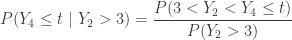
Draw a random sample $X_1,X_2,X_3,X_4,X_5$ from the uniform distribution $U(0,5)$ . The resulting order statistics are $Y_1<Y_2<Y_3<Y_4 <Y_5$ . Consider the conditional random variable $Y_4 \ | \ Y_2 >3$ . For this conditional distribution, find the following:

$P( Y_4 \le t \ | \ Y_2 >3)$
$f_{Y_4}(t \ | \ Y_2 >3)$
$E(Y_4 \ | \ Y_2 >3)$

where $3<t<5$ . Note that $f_{Y_4}(t | \ Y_2 >3)$ is the density function of $Y_4 \ | \ Y_2 >3$ .

Note that

$\displaystyle P( Y_4 \le t \ | \ Y_2 >3)=\frac{P(3<Y_2<Y_4 \le t)}{P(Y_2 >3)}$

In finding $P(3<Y_2<Y_4 \le t)$ , the range (0, 5) is broken up into 3 intervals (0, 3), (3, t) and (t, 5). The sample items fall into these intervals with probabilities $\frac{3}{5}$ , $\frac{t-3}{5}$ and $\frac{5-t}{5}$ .

Since $Y_2 >3$ , there is at most 1 sample item in the interval (0, 3). Since $Y_4 \le t$ , there are at least 4 sample items in the interval (0, t). So the count in the interval (3, t) and the count in (0, 3) should add up to 4 or more items. The following shows all the cases for the event $3<Y_2<Y_4 \le t$ along with the corresponding multinomial probabilities.

$\displaystyle [0, 4, 1] \ \ \ \ \ \ \frac{5!}{0! \ 4! \ 1!} \ \biggl[\frac{3}{5} \biggr]^0 \ \biggl[\frac{t-3}{5} \biggr]^4 \ \biggl[\frac{5-t}{5} \biggr]^1$

$\displaystyle [0, 5, 0] \ \ \ \ \ \ \frac{5!}{0! \ 5! \ 0!} \ \biggl[\frac{3}{5} \biggr]^0 \ \biggl[\frac{t-3}{5} \biggr]^5 \ \biggl[\frac{5-t}{5} \biggr]^0$

$\displaystyle [1, 3, 1] \ \ \ \ \ \ \frac{5!}{1! \ 3! \ 1!} \ \biggl[\frac{3}{5} \biggr]^1 \ \biggl[\frac{t-3}{5} \biggr]^3 \ \biggl[\frac{5-t}{5} \biggr]^1$

$\displaystyle [1, 4, 0] \ \ \ \ \ \ \frac{5!}{1! \ 4! \ 0!} \ \biggl[\frac{3}{5} \biggr]^1 \ \biggl[\frac{t-3}{5} \biggr]^4 \ \biggl[\frac{5-t}{5} \biggr]^0$

After carrying the algebra and simplifying, we have the following:

$\displaystyle P(3<Y_2<Y_4 \le t)=\frac{-4t^5+25t^4+180t^3-1890t^2+5400t-5103}{3125}$

For the event $Y_2 >3$ to happen, there is at most 1 sample item less than 3. So we have:

$\displaystyle P(Y_2 >3)=\binom{5}{0} \ \biggl[\frac{3}{5} \biggr]^0 \ \biggl[\frac{2}{5} \biggr]^5 +\binom{5}{1} \ \biggl[\frac{3}{5} \biggr]^1 \ \biggl[\frac{2}{5} \biggr]^4=\frac{272}{3125}$

$\displaystyle P( Y_4 \le t \ | \ Y_2 >3)=\frac{-4t^5+25t^4+180t^3-1890t^2+5400t-5103}{272}$

Then the conditional density is obtained by differentiating $P( Y_4 \le t \ | \ Y_2 >3)$ .

$\displaystyle f_{Y_4}(t \ | \ Y_2 >3)=\frac{-20t^4+100t^3+540t^2-3750t+5400}{272}$

The following gives the conditional mean $E(Y_4 \ | \ Y_2 >3)$ .

$\displaystyle \begin{aligned} E(Y_4 \ | \ Y_2 >3)&=\frac{1}{272} \ \int_3^5 t(-20t^4+100t^3+540t^2-3750t+5400) \ dt \\&=\frac{215}{51}=4.216 \end{aligned}$

To contrast, the following gives the information on the unconditional distribution of $Y_4$ .

$\displaystyle f_{Y_4}(t)=\frac{5!}{3! \ 1! \ 1!} \ \biggl[\frac{t}{5} \biggr]^3 \ \biggl[\frac{1}{5} \biggr] \ \biggl[ \frac{5-t}{5} \biggr]^1=\frac{20}{3125} \ (5t^3-t^4)$

$\displaystyle E(Y_4)=\frac{20}{3125} \ \int_0^5 t(5t^3-t^4) \ dt=\frac{10}{3}=3.33$

The unconditional mean of $Y_4$ is about 3.33. With the additional information that $Y_2 >3$ , the average of $Y_4$ is now 4.2. So a higher value of $Y_2$ pulls up the mean of $Y_4$ .

________________________________________________________________________

Practice problems

Practice problems to reinforce the calculation are found in the problem blog, a companion blog to this blog.

________________________________________________________________________
$\copyright \ \text{2015 by Dan Ma}$

A Blog on Probability and Statistics

Calculating order statistics using multinomial probabilities

1 thought on “Calculating order statistics using multinomial probabilities”

Leave a reply to Wicky Cancel reply

Share this:

Related

1 thought on “Calculating order statistics using multinomial probabilities”

Leave a reply to Wicky Cancel reply