The Gamma Function

A student in a probability course may have evaluated an integral such as the following:

$\displaystyle \int_0^\infty \displaystyle t^{x-1} \ e^{-t} \ dt$

Plug in a value for $x$ and evaluate the integral. For example, when evaluated at $x=1$ , the integral has value 1. Evaluated at $x=2$ , the result is also 1. Evaluated at $x=3$ , the result is 2. At $x=4$ , the result is 6=3!. In fact, if a student remembers a fact about this function (called the gamma function), it is that it gives the factorial when evaluated at the positive integers – the value of the integral is $(x-1)!$ when evaluated at the positive integer $x$ .

$\displaystyle (1) \ \ \ \ \ \Gamma(x)=\int_0^\infty \displaystyle t^{x-1} \ e^{-t} \ dt$

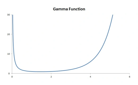
The gamma function is denoted by the capital Greek letter $\Gamma$ . It crops up almost everywhere in mathematics. It has applications in many branches of mathematics including probability and statistics. The integral described above may seem inconsequential, no more than an exercise in an undergraduate course on probability and statistics. We give ample evidence that the gamma function is indeed very consequential, even just in the area of statistics. Our brief tour is through the gamma distribution, a probability distribution that naturally arises from the gamma function. Most of the material cited here is written in various affiliated blogs. Anyone who wants to check out the details can refer to those blogs. Links will be given at the appropriate places.

The Gamma Function

The starting point of the gamma function is that $\Gamma(x)$ is defined for $x>0$ according to the integral described above. A natural question: how do we know that the integral converges, i.e. the integral always gives a valid number as result? How do we know that the integral does not give infinity as result? The integral does converge for all $x>0$ . A proof can be found here. The following is a graph of the gamma function (using Excel).

Gamma Function Graph

As indicated above, the function gives the value of the factorial shifted down by one, i.e. $\Gamma(x)=(x-1)!$ . Thus the graph of the gamma function goes up without bound as $x \rightarrow \infty$ .

It is easy to evaluate $\Gamma(1)$ . To evaluate the function at the higher integers, the integral would required integration by parts. In fact, using integration by parts, the following recursive relation is established.

$(2a) \ \ \ \ \ \Gamma(x+1)=x \Gamma(x)$

$\displaystyle (2b) \ \ \ \ \ \Gamma(x)=\frac{\Gamma(x+1)}{x}$

The recursive relation works for all real numbers $x>0$ , not just the integers. For example, knowing that $\Gamma(\frac{1}{2})=\sqrt{\pi}$ , we have $\Gamma(\frac{3}{2})=\frac{1}{2} \sqrt{\pi}$ . Furthermore, the relation (2b) gives a way to extend the gamma function to the negative numbers. For example, $\Gamma(-\frac{1}{2})$ would be evaluated by $\frac{\Gamma(\frac{1}{2})}{-\frac{1}{2}}=-2 \Gamma(\frac{1}{2})$ . Based on this idea, for any real number in the interval $(-1,0)$ , $\Gamma(x)$ would be defined using the relation (2b) and would be a negative value.

The idea can be extended further. For example, for any real number in the interval $(-2,-1)$ , $\Gamma(x)$ would be defined using the relation (2b) and would be a positive value (since the previous interval gives negative values). Continue in this same manner, $\Gamma(x)$ is defined for all negative real numbers except for the negative integers and zero. The following is a graph of the gamma function over all of the real number line.

Gamma Function

The gamma function can also be extended to the complex numbers. Thus the gamma function is defined on all real numbers (except for zero and the negative integers) and on all complex numbers.

Gamma Distribution

We are now back to looking at the gamma function just on the positive real numbers $x>0$ . Instead of using $x$ as the argument of the function, let’s use the Greek letter $\alpha$ .

$\displaystyle (1) \ \ \ \ \ \Gamma(\alpha)=\int_0^\infty \displaystyle x^{\alpha-1} \ e^{-x} \ dx$

Let’s look at the graph of the integrand of the gamma function defined in (1). In particular, look at $\Gamma(5)$ , which is 4! = 24. The integrand would be the expression $x^4 \ e^{-x}$ . Let’s graph this expression over all $t>0$ .

Integrand of Gamma Function: area under curve is 24

The above graph is the graph of $y=x^4 \ e^{-x}$ for $x>0$ . One thing of interest is that the area under the graph (and above the x-axis) is 24 since the gamma function evaluated at 5 is 4!. What if we divide the integrand by 24? Let’s graph the expression $y=\frac{1}{24} \ x^4 \ e^{-x}$ .

Integrand of Gamma Function: area under curve is 1

Note that the graph of $y=\frac{1}{24} \ x^4 \ e^{-x}$ has the same shape as the previous one without the multiplier $\frac{1}{24}$ . The second curve is just a compression of the first one. But this time the area under the curve is 1. This means that $y=\frac{1}{24} \ x^4 \ e^{-x}$ is a probability density function for a random variable that takes on positive values. There is nothing special about $\Gamma(5)$ . The same compression can be done for any $\Gamma(\alpha)$ . The following is always a probability density function.

$\displaystyle (3) \ \ \ \ \ f_X(x)=\frac{1}{\Gamma(\alpha)} \ x^{\alpha-1} \ e^{-x}$

where $x>0$ and $\alpha>0$ . The number $\alpha$ is a parameter of the distribution. Since this is derived from the gamma function, it is called the gamma distribution. The distribution described in (3) is not the full picture. It has only one parameter $\alpha$ , the shape parameter. We can add another parameter $\theta$ to work as a scale parameter.

$\displaystyle (4) \ \ \ \ \ f_X(x)=\frac{1}{\Gamma(\alpha)} \ \frac{1}{\theta^\alpha} \ x^{\alpha-1} \ e^{-x/\theta}$

where $x>0$ , $\alpha>0$ and $\theta>0$ . Thus the gamma distribution has two parameters $\alpha$ (the shape parameter) and $\theta$ (the scale parameter).

The mathematical definition of the gamma distribution is quite simple. Once the gamma function is understood, the gamma distribution is clear mathematically speaking. The mathematical properties of the gamma function is discussed here in a companion blog. The gamma distribution is defined in this blog post in the same companion blog.

Beyond the Mathematical Definition

Though the definition may be simple, the impact of the gamma distribution is far reaching and enormous. We give a few indications. The gamma distribution is useful in actuarial modeling, e.g. modeling insurance losses. Due to its mathematical properties, there is considerable flexibility in the modeling process. For example, since it has two parameters (a scale parameter and a shape parameter), the gamma distribution is capable of representing a variety of distribution shapes and dispersion patterns.

The exponential distribution is a special case of the gamma distribution and it arises naturally as the waiting time between two events in a Poisson process (see here and here).

The chi-squared distribution is also a sub family of the gamma family of distributions. Mathematically speaking, a chi-squared distribution is a gamma distribution with shape parameter $k/2$ and scale parameter 2 with $k$ being a positive integer (called the degrees of freedom). Though the definition is simple mathematically, the chi-squared family plays an outsize role in statistics.

This blog post discusses the chi-square distribution from a mathematical standpoint. The chi-squared distribution also play important roles in inferential statistics for the population mean and population variance of normal populations (discussed here).

The chi-squared distribution also figures prominently in the inference on categorical data. The chi-squared test, based on the chi-squared distribution, is used to determine whether there is a significant difference between the expected frequencies and the observed frequencies in one or more categories. The chi-squared test is based on the chi-squared statistic, which has three different interpretations – goodness-of-fit test, test of homogeneity and test of independence.Further discussion of the chi-squared test is found here.

Another set of distributions that are derived from the gamma family is through raising a gamma distribution to a power. Raising a gamma distribution to a positive power results in a transformed gamma distribution. Raising a gamma distribution to -1 results in an inverse gamma distribution. Raising a gamma distribution to a negative power not -1 results in an inverse transformed gamma distribution. These derived distributions greatly expand the tool kit for actuarial modeling. These distributions are discussed here.

The applications discussed here and in the companion blogs are just scratch the surface on the subject of gamma function and gamma distribution. One thing is clear, the one little integral in (1) above has a far and wide reach in mathematics, statistics and engineering and other fields.

$\text{ }$

A Blog on Probability and Statistics

The Gamma Function

Leave a comment Cancel reply

Share this:

Related

Leave a comment Cancel reply