
We present more examples to further illustrate the thought process of conditional distributions. A conditional distribution is a probability distribution derived from a given probability distribution by focusing on a subset of the original sample space (we assume that the probability distribution being discussed is a model for some random experiment). The new sample space (the subset of the original one) may be some outcomes that are of interest to an experimenter in a random experiment or may reflect some new information we know about the random experiment in question. We illustrate this thought process in the previous post Conditional Distributions, Part 1 using discrete distributions. In this post, we present some continuous examples for conditional distributions. One concept illustrated by the examples in this post is the notion of mean residual life, which has an insurance interpretation (e.g. the average remaining time until death given that the life in question is alive at a certain age).
_____________________________________________________________________________________________________________________________
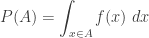
The Setting
The thought process of conditional distributions is discussed in the previous post Conditional Distributions, Part 1. We repeat the same discussion using continuous distributions.
Let 


We assume that 

Suppose that in the random experiment in question, certain event 
Since the event 


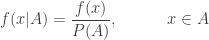
The above probability distribution is called the conditional distribution of 
Once this new probability distribution is established, we can compute various distributional quantities (e.g. cumulative distribution function, mean, variance and other higher moments).
_____________________________________________________________________________________________________________________________
Examples
Example 1
Let

Suppose that you have just purchased a one such computer that is 2-year old and in good working condition. We have the following questions.
- What is the expected lifetime of this 2-year old computer?
- What is the expected number of years of service that will be provided by this 2-year old computer?
Both calculations are conditional means since the computer in question already survived to age 2. However, there is a slight difference between the two calculations. The first one is the expected age of the 2-year old computer, i.e., the conditional mean 

For a brand new computer, the sample space is the interval 


The conditional density function of 

The first conditional mean is:
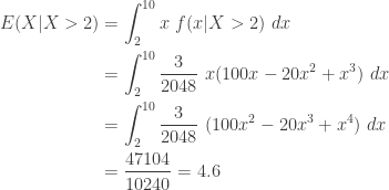
The second conditional mean is:

In contrast, the unconditional mean is:

So if the lifetime of a computer is modeled by the density function
Note that the following calculation is not

The above calculation does not use the conditional distribution that 
Example 2 – Exponential Distribution
Work Example 1 again by assuming that the lifetime of the type of computers in questions follows the exponential distribution with mean 4 years.
The following is the density function of the lifetime

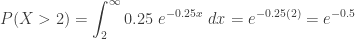
The probability that the computer has survived to age 2 is:
The conditional density function given that

To compute the conditional mean

Then 
We have an interesting result here. The expected lifetime of a brand new computer is 4 years. Yet the remaining lifetime for a 2-year old computer is still 4 years! This is the no-memory property of the exponential distribution – if the lifetime of a type of machines is distributed according to an exponential distribution, it does not matter how old the machine is, the remaining lifetime is always the same as the unconditional mean! This point indicates that the exponential distribution is not an appropriate for modeling the lifetime of machines or biological lives that wear out over time.
_____________________________________________________________________________________________________________________________
Mean Residual Life
If a 40-year old man who is a non-smoker wants to purchase a life insurance policy, the insurance company is interested in knowing the expected remaining lifetime of the prospective policyholder. This information will help determine the pricing of the life insurance policy. The expected remaining lifetime of the prospective policyholder is called is called the mean residual life and is the conditional mean 
In engineering and manufacturing applications, probability modeling of lifetimes of objects (e.g. devices, systems or machines) is known as reliability theory. The mean residual life also plays an important role in such applications.
Thus if the random variable 
On the other hand, if the random variable
_____________________________________________________________________________________________________________________________
Summary
In conclusion, we summarize the approach for calculating the two conditional means demonstrated in the above examples.
Suppose 


Then we have the two conditional means:


If 

If
_____________________________________________________________________________________________________________________________
Practice Problems
Practice problems are found in the companion blog.
_____________________________________________________________________________________________________________________________

 as the probability mass function. Suppose some random experiment can be modeled by the discrete random variable
  for which
  . In the examples below,
  . Conceivably the sample space could be subset of any Euclidean space
  in higher dimension.
 , is derived by summing the probabilities
  . We have:
 or divided by 0.5) and the second probability mass is 0.6.
 be the number of correct answers of the other student (these can be considered as test scores for the purpose of the examples here). Assume that
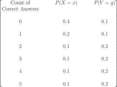
 and
and  . Without knowing any additional information, we can expect on average one student gets 1.6 correct answers and one student gets 2.9 correct answers. If having 3 or more correct answers is considered passing, then the student represented by
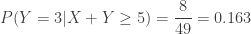
  , we also know that this student has at least one correct answer (i.e. the new information is
  ).
). . Note that
  . In this new sample space, each probability mass is the original one divided by 0.6. For example, for the sample point
  , we have
 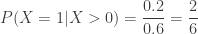 . The following is the conditional probability distribution of


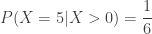
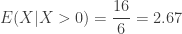 . Given that this student is knowledgeable enough to answer some question correctly, the expectation is higher than before knowing the additional information. Also, given the new information, the student in question has a 50% chance of passing (vs. 30% before the new information is known).

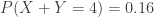
 . The following figure shows one such joint probability.

 and the conditional probability distribution of
  . In particular, given that there are 4 correct answers between the two students, what would be their expected numbers of correct answers and what would be their chances of passing?


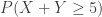
 . Making each of these joint probabilities as a fraction of 0.16, we have the following two conditional probability distributions.


 , comparing against the unconditional means.


 increases to 0.5 from 0.4, while the conditional probability at
  increases to 0.5 from 0.2.
 . How would this impact the conditional distributions?
 and
and  . By considering the new information, the following is the new sample space.
 . The calculation is shown below.


 . The conditional distribution of
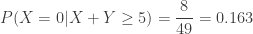


 (vs.
(vs.  (vs.
(vs.  ).
). 


 (vs.
(vs.  (vs.
(vs. 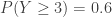 ). Indeed, with the information that both test takers do well, we can expect much higher results from each individual test taker.
 . Then what is the conditional distribution for
  ? Since
  .
.