A counting distribution is a discrete distribution with probabilities only on the nonnegative integers. Such distributions are important in insurance applications since they can be used to model the number of events such as losses to the insured or claims to the insurer. Though playing a prominent role in statistical theory, the Poisson distribution is not appropriate in all situations, since it requires that the mean and the variance are equaled. Thus the negative binomial distribution is an excellent alternative to the Poisson distribution, especially in the cases where the observed variance is greater than the observed mean.
The negative binomial distribution arises naturally from a probability experiment of performing a series of independent Bernoulli trials until the occurrence of the rth success where r is a positive integer. From this starting point, we discuss three ways to define the distribution. We then discuss several basic properties of the negative binomial distribution. Emphasis is placed on the close connection between the Poisson distribution and the negative binomial distribution.
________________________________________________________________________
Definitions
We define three versions of the negative binomial distribution. The first two versions arise from the view point of performing a series of independent Bernoulli trials until the rth success where r is a positive integer. A Bernoulli trial is a probability experiment whose outcome is random such that there are two possible outcomes (success or failure).
Let  be the number of Bernoulli trials required for the rth success to occur where r is a positive integer. Let
  is the probability of success in each trial. The following is the probability function of :

The idea for  is that for
  to happen, there must be
  successes in the first
  trials and one additional success occurring in the last trial (the
  th trial).
A more common version of the negative binomial distribution is the number of Bernoulli trials in excess of r in order to produce the rth success. In other words, we consider the number of failures before the occurrence of the rth success. Let  be this random variable. The following is the probability function of :

The idea for  is that there are
  trials and in the first
  trials, there are failures (or equivalently successes).
In both and , the binomial coefficient is defined by
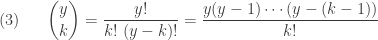
where  is a positive integer and
  is a nonnegative integer. However, the right-hand-side of
  can be calculated even if is not a positive integer. Thus the binomial coefficient
  can be expanded to work for all real number . However must still be nonnegative integer.

For convenience, we let  . When the real number
  , the binomial coefficient in
  can be expressed as:
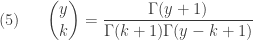
where  is the gamma function.
With the more relaxed notion of binomial coefficient, the probability function in above can be defined for all real number r. Thus the general version of the negative binomial distribution has two parameters r and , both real numbers, such that  . The following is its probability function.

Whenever r in  is a real number that is not a positive integer, the interpretation of counting the number of failures until the occurrence of the rth success is no longer important. Instead we can think of it simply as a count distribution.
The following alternative parametrization of the negative binomial distribution is also useful.

The parameters in this alternative parametrization are r and  . Clearly, the ratio
  takes the place of in . Unless stated otherwise, we use the parametrization of .
________________________________________________________________________
What is negative about the negative binomial distribution?
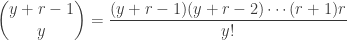
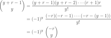
What is negative about this distribution? What is binomial about this distribution? The name is suggested by the fact that the binomial coefficient in can be rearranged as follows:

The calculation in  can be used to verify that is indeed a probability function, that is, all the probabilities sum to 1.
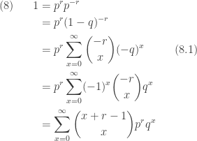
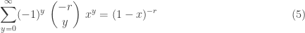
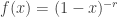
In  , we take
  . The step
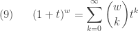
  above uses the following formula known as the Newton’s binomial formula.
For a detailed discussion of (8) with all the details worked out, see the post called Deriving some facts of the negative binomial distribution.
________________________________________________________________________
The Generating Function
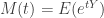
By definition, the following is the generating function of the negative binomial distribution, using :

where . Using a similar calculation as in , the generating function can be simplified as:

As a result, the moment generating function of the negative binomial distribution is:
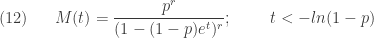
For a detailed discussion of (12) with all the details worked out, see the post called Deriving some facts of the negative binomial distribution.
________________________________________________________________________
Independent Sum
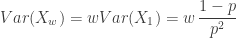
One useful property of the negative binomial distribution is that the independent sum of negative binomial random variables, all with the same parameter , also has a negative binomial distribution. Let  be an independent sum such that each
  has a negative binomial distribution with parameters
  and . Then the sum has a negative binomial distribution with parameters
  and .
and .
Note that the generating function of an independent sum is the product of the individual generating functions. The following shows that the product of the individual generating functions is of the same form as  , thus proving the above assertion.

________________________________________________________________________
Mean and Variance
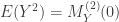
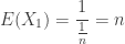
The mean and variance can be obtained from the generating function. From  and
and  , we have:

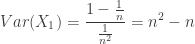
Note that  . Thus when the sample data suggest that the variance is greater than the mean, the negative binomial distribution is an excellent alternative to the Poisson distribution. For example, suppose that the sample mean and the sample variance are 3.6 and 7.1. In exploring the possibility of fitting the data using the negative binomial distribution, we would be interested in the negative binomial distribution with this mean and variance. Then plugging these into
  produces the negative binomial distribution with
  and
and  .
.
________________________________________________________________________
The Poisson-Gamma Mixture
One important application of the negative binomial distribution is that it is a mixture of a family of Poisson distributions with Gamma mixing weights. Thus the negative binomial distribution can be viewed as a generalization of the Poisson distribution. The negative binomial distribution can be viewed as a Poisson distribution where the Poisson parameter is itself a random variable, distributed according to a Gamma distribution. Thus the negative binomial distribution is known as a Poisson-Gamma mixture.
In an insurance application, the negative binomial distribution can be used as a model for claim frequency when the risks are not homogeneous. Let  has a Poisson distribution with parameter
  , which can be interpreted as the number of claims in a fixed period of time from an insured in a large pool of insureds. There is uncertainty in the parameter , reflecting the risk characteristic of the insured. Some insureds are poor risks (with large ) and some are good risks (with small ). Thus the parameter should be regarded as a random variable
  . The following is the conditional distribution of the random variable (conditional on
  ):
):

Suppose that has a Gamma distribution with scale parameter  and shape parameter
  . The following is the probability density function of .

Then the joint density of and is:

The unconditional distribution of is obtained by summing out in  .
.
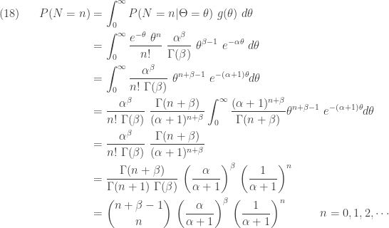
Note that the integral in the fourth step in  is 1.0 since the integrand is the pdf of a Gamma distribution. The above probability function is that of a negative binomial distribution. It is of the same form as
  . Equivalently, it is also of the form with parameter
  and
and  .
.
The variance of the negative binomial distribution is greater than the mean. In a Poisson distribution, the mean equals the variance. Thus the unconditional distribution of is more dispersed than its conditional distributions. This is a characteristic of mixture distributions. The uncertainty in the parameter variable has the effect of increasing the unconditional variance of the mixture distribution of . The variance of a mixture distribution has two components, the weighted average of the conditional variances and the variance of the conditional means. The second component represents the additional variance introduced by the uncertainty in the parameter (see The variance of a mixture).
________________________________________________________________________
The Poisson Distribution as Limit of Negative Binomial
There is another connection to the Poisson distribution, that is, the Poisson distribution is a limiting case of the negative binomial distribution. We show that the generating function of the Poisson distribution can be obtained by taking the limit of the negative binomial generating function as  . Interestingly, the Poisson distribution is also the limit of the binomial distribution.
In this section, we use the negative binomial parametrization of . By replacing for , the following are the mean, variance, and the generating function for the probability function in :
![\displaystyle \begin{aligned}(19) \ \ \ \ \ \ &E(X)=\frac{r}{\alpha} \\&\text{ }\\&Var(X)=\frac{\alpha+1}{\alpha} \ \frac{r}{\alpha}=\frac{r(\alpha+1)}{\alpha^2} \\&\text{ } \\&g(z)=\frac{1}{[1-\frac{1}{\alpha}(z-1)]^r} \ \ \ \ \ \ \ z<\alpha+1 \end{aligned}](https://s0.wp.com/latex.php?latex=%5Cdisplaystyle+%5Cbegin%7Baligned%7D%2819%29+%5C+%5C+%5C+%5C+%5C+%5C+%26E%28X%29%3D%5Cfrac%7Br%7D%7B%5Calpha%7D+%5C%5C%26%5Ctext%7B+%7D%5C%5C%26Var%28X%29%3D%5Cfrac%7B%5Calpha%2B1%7D%7B%5Calpha%7D+%5C+%5Cfrac%7Br%7D%7B%5Calpha%7D%3D%5Cfrac%7Br%28%5Calpha%2B1%29%7D%7B%5Calpha%5E2%7D+%5C%5C%26%5Ctext%7B+%7D+%5C%5C%26g%28z%29%3D%5Cfrac%7B1%7D%7B%5B1-%5Cfrac%7B1%7D%7B%5Calpha%7D%28z-1%29%5D%5Er%7D+%5C+%5C+%5C+%5C+%5C+%5C+%5C+z%3C%5Calpha%2B1+%5Cend%7Baligned%7D&bg=ffffff&fg=333333&s=0&c=20201002)
Let r goes to infinity and  goes to zero and at the same time keeping their product constant. Thus
  is constant (this is the mean of the negative binomial distribution). We show the following:
![\displaystyle (20) \ \ \ \ \ \lim \limits_{r \rightarrow \infty} [1-\frac{\mu}{r}(z-1)]^{-r}=e^{\mu (z-1)}](https://s0.wp.com/latex.php?latex=%5Cdisplaystyle+%2820%29+%5C+%5C+%5C+%5C+%5C+%5Clim+%5Climits_%7Br+%5Crightarrow+%5Cinfty%7D+%5B1-%5Cfrac%7B%5Cmu%7D%7Br%7D%28z-1%29%5D%5E%7B-r%7D%3De%5E%7B%5Cmu+%28z-1%29%7D&bg=ffffff&fg=333333&s=0&c=20201002)
The right-hand side of  is the generating function of the Poisson distribution with mean
  . The generating function in the left-hand side is that of a negative binomial distribution with mean . The following is the derivation of .
![\displaystyle \begin{aligned}(21) \ \ \ \ \ \lim \limits_{r \rightarrow \infty} [1-\frac{\mu}{r}(z-1)]^{-r}&=\lim \limits_{r \rightarrow \infty} e^{\displaystyle \biggl(ln[1-\frac{\mu}{r}(z-1)]^{-r}\biggr)} \\&=\lim \limits_{r \rightarrow \infty} e^{\displaystyle \biggl(-r \ ln[1-\frac{\mu}{r}(z-1)]\biggr)} \\&=e^{\displaystyle \biggl(\lim \limits_{r \rightarrow \infty} -r \ ln[1-\frac{\mu}{r}(z-1)]\biggr)} \end{aligned}](https://s0.wp.com/latex.php?latex=%5Cdisplaystyle+%5Cbegin%7Baligned%7D%2821%29+%5C+%5C+%5C+%5C+%5C+%5Clim+%5Climits_%7Br+%5Crightarrow+%5Cinfty%7D+%5B1-%5Cfrac%7B%5Cmu%7D%7Br%7D%28z-1%29%5D%5E%7B-r%7D%26%3D%5Clim+%5Climits_%7Br+%5Crightarrow+%5Cinfty%7D+e%5E%7B%5Cdisplaystyle+%5Cbiggl%28ln%5B1-%5Cfrac%7B%5Cmu%7D%7Br%7D%28z-1%29%5D%5E%7B-r%7D%5Cbiggr%29%7D+%5C%5C%26%3D%5Clim+%5Climits_%7Br+%5Crightarrow+%5Cinfty%7D+e%5E%7B%5Cdisplaystyle+%5Cbiggl%28-r+%5C+ln%5B1-%5Cfrac%7B%5Cmu%7D%7Br%7D%28z-1%29%5D%5Cbiggr%29%7D+%5C%5C%26%3De%5E%7B%5Cdisplaystyle+%5Cbiggl%28%5Clim+%5Climits_%7Br+%5Crightarrow+%5Cinfty%7D+-r+%5C+ln%5B1-%5Cfrac%7B%5Cmu%7D%7Br%7D%28z-1%29%5D%5Cbiggr%29%7D+%5Cend%7Baligned%7D&bg=ffffff&fg=333333&s=0&c=20201002)
We now focus on the limit in the exponent.
![\displaystyle \begin{aligned}(22) \ \ \ \ \ \lim \limits_{r \rightarrow \infty} -r \ ln[1-\frac{\mu}{r}(z-1)]&=\lim \limits_{r \rightarrow \infty} \frac{ln(1-\frac{\mu}{r} (z-1))^{-1}}{r^{-1}} \\&=\lim \limits_{r \rightarrow \infty} \frac{(1-\frac{\mu}{r} (z-1)) \ \mu (z-1) r^{-2}}{r^{-2}} \\&=\mu (z-1) \end{aligned}](https://s0.wp.com/latex.php?latex=%5Cdisplaystyle+%5Cbegin%7Baligned%7D%2822%29+%5C+%5C+%5C+%5C+%5C+%5Clim+%5Climits_%7Br+%5Crightarrow+%5Cinfty%7D+-r+%5C+ln%5B1-%5Cfrac%7B%5Cmu%7D%7Br%7D%28z-1%29%5D%26%3D%5Clim+%5Climits_%7Br+%5Crightarrow+%5Cinfty%7D+%5Cfrac%7Bln%281-%5Cfrac%7B%5Cmu%7D%7Br%7D+%28z-1%29%29%5E%7B-1%7D%7D%7Br%5E%7B-1%7D%7D+%5C%5C%26%3D%5Clim+%5Climits_%7Br+%5Crightarrow+%5Cinfty%7D+%5Cfrac%7B%281-%5Cfrac%7B%5Cmu%7D%7Br%7D+%28z-1%29%29+%5C+%5Cmu+%28z-1%29+r%5E%7B-2%7D%7D%7Br%5E%7B-2%7D%7D+%5C%5C%26%3D%5Cmu+%28z-1%29+%5Cend%7Baligned%7D&bg=ffffff&fg=333333&s=0&c=20201002)
The middle step in  uses the L’Hopital’s Rule. The result in is obtained by combining
  and .
and .
________________________________________________________________________
Reference
- Klugman S.A., Panjer H. H., Wilmot G. E. Loss Models, From Data to Decisions, Second Edition., Wiley-Interscience, a John Wiley & Sons, Inc., New York, 2004
________________________________________________________________________


 the number of Bernoulli trials required to get the
  the number of Bernoulli trials that end in failure before getting the


![\displaystyle \begin{aligned} M(t)&=E(e^{tY}) \\&=\sum \limits_{y=0}^\infty \ e^{t y} \ \binom{y+r-1}{y} \ p^r \ (1-p)^y \\&=p^r \ \sum \limits_{y=0}^\infty \ \binom{y+r-1}{y} \ [(1-p) e^t]^y \\&=p^r \ \sum \limits_{y=0}^\infty \ (-1)^y \binom{-r}{y} \ [(1-p) e^t]^y \ \ \ \ \ \ \ \ \ \ \ \text{using } (4) \\&=p^r \ [1-(1-p) \ e^t]^{-r} \ \ \ \ \ \ \ \ \ \ \ \ \ \ \ \ \ \ \ \ \ \ \ \ \ \ \text{using } (5) \\&=\frac{p^r}{[1-(1-p) \ e^t]^{r}}\end{aligned}](https://s0.wp.com/latex.php?latex=%5Cdisplaystyle+%5Cbegin%7Baligned%7D+M%28t%29%26%3DE%28e%5E%7BtY%7D%29+%5C%5C%26%3D%5Csum+%5Climits_%7By%3D0%7D%5E%5Cinfty+%5C+e%5E%7Bt+y%7D+%5C+%5Cbinom%7By%2Br-1%7D%7By%7D+%5C+p%5Er+%5C+%281-p%29%5Ey+%5C%5C%26%3Dp%5Er+%5C+%5Csum+%5Climits_%7By%3D0%7D%5E%5Cinfty++%5C+%5Cbinom%7By%2Br-1%7D%7By%7D+%5C+%5B%281-p%29+e%5Et%5D%5Ey+%5C%5C%26%3Dp%5Er+%5C+%5Csum+%5Climits_%7By%3D0%7D%5E%5Cinfty++%5C+%28-1%29%5Ey+%5Cbinom%7B-r%7D%7By%7D+%5C+%5B%281-p%29+e%5Et%5D%5Ey+%5C+%5C+%5C+%5C+%5C+%5C+%5C+%5C+%5C+%5C+%5C+%5Ctext%7Busing+%7D+%284%29+%5C%5C%26%3Dp%5Er+%5C+%5B1-%281-p%29+%5C+e%5Et%5D%5E%7B-r%7D+%5C+%5C+%5C+%5C+%5C+%5C+%5C+%5C+%5C+%5C+%5C+%5C+%5C+%5C+%5C+%5C+%5C+%5C+%5C+%5C+%5C+%5C+%5C+%5C+%5C+%5C+%5Ctext%7Busing+%7D+%285%29+%5C%5C%26%3D%5Cfrac%7Bp%5Er%7D%7B%5B1-%281-p%29+%5C+e%5Et%5D%5E%7Br%7D%7D%5Cend%7Baligned%7D&bg=ffffff&fg=333333&s=0&c=20201002)


![\displaystyle M_X(t)=E[e^{tX}]=\frac{p^r \ e^{tr}}{[1-(1-p) \ e^t]^{r}} \ \ \ \ \ \ \ \ \ \ \ \ \ \ \ \ \text{for } (1)](https://s0.wp.com/latex.php?latex=%5Cdisplaystyle+M_X%28t%29%3DE%5Be%5E%7BtX%7D%5D%3D%5Cfrac%7Bp%5Er+%5C+e%5E%7Btr%7D%7D%7B%5B1-%281-p%29+%5C+e%5Et%5D%5E%7Br%7D%7D+%5C+%5C+%5C+%5C+%5C+%5C+%5C+%5C+%5C+%5C+%5C+%5C+%5C+%5C+%5C+%5C+%5Ctext%7Bfor+%7D+%281%29&bg=ffffff&fg=333333&s=0&c=20201002)
![\displaystyle M_Y(t)=E[e^{tY}]=\frac{p^r}{[1-(1-p) \ e^t]^{r}} \ \ \ \ \ \ \ \ \ \ \ \ \ \ \ \ \text{for } (2) \text{ and } (3)](https://s0.wp.com/latex.php?latex=%5Cdisplaystyle+M_Y%28t%29%3DE%5Be%5E%7BtY%7D%5D%3D%5Cfrac%7Bp%5Er%7D%7B%5B1-%281-p%29+%5C+e%5Et%5D%5E%7Br%7D%7D+%5C+%5C+%5C+%5C+%5C+%5C+%5C+%5C+%5C+%5C+%5C+%5C+%5C+%5C+%5C+%5C+%5Ctext%7Bfor+%7D+%282%29+%5Ctext%7B+and+%7D+%283%29&bg=ffffff&fg=333333&s=0&c=20201002)


![\displaystyle E(Y^2)=\frac{r(1-p)[1+(1-p)]}{p^2}](https://s0.wp.com/latex.php?latex=%5Cdisplaystyle+E%28Y%5E2%29%3D%5Cfrac%7Br%281-p%29%5B1%2B%281-p%29%5D%7D%7Bp%5E2%7D&bg=ffffff&fg=333333&s=0&c=20201002)
![\displaystyle \begin{aligned} Var(Y)&=E(Y^2)-E(Y)^2 \\&=\frac{r(1-p)[1+(1-p)]}{p^2}-\frac{(1-p)^2}{p^2} \\&=\frac{r(1-p)[1+r(1-p)-r(1-p)]}{p^2} \\&=\frac{r(1-p)}{p^2} \end{aligned}](https://s0.wp.com/latex.php?latex=%5Cdisplaystyle+%5Cbegin%7Baligned%7D+Var%28Y%29%26%3DE%28Y%5E2%29-E%28Y%29%5E2+%5C%5C%26%3D%5Cfrac%7Br%281-p%29%5B1%2B%281-p%29%5D%7D%7Bp%5E2%7D-%5Cfrac%7B%281-p%29%5E2%7D%7Bp%5E2%7D+%5C%5C%26%3D%5Cfrac%7Br%281-p%29%5B1%2Br%281-p%29-r%281-p%29%5D%7D%7Bp%5E2%7D+%5C%5C%26%3D%5Cfrac%7Br%281-p%29%7D%7Bp%5E2%7D++%5Cend%7Baligned%7D&bg=ffffff&fg=333333&s=0&c=20201002)


![\displaystyle M_T(t)=E[e^{tT}]=\frac{p^g}{[1-(1-p) \ e^t]^{g}}](https://s0.wp.com/latex.php?latex=%5Cdisplaystyle+M_T%28t%29%3DE%5Be%5E%7BtT%7D%5D%3D%5Cfrac%7Bp%5Eg%7D%7B%5B1-%281-p%29+%5C+e%5Et%5D%5E%7Bg%7D%7D&bg=ffffff&fg=333333&s=0&c=20201002)


![\displaystyle M_W(t)=E[e^{tW}]=\frac{p^n}{[1-(1-p) \ e^t]^{n}}](https://s0.wp.com/latex.php?latex=%5Cdisplaystyle+M_W%28t%29%3DE%5Be%5E%7BtW%7D%5D%3D%5Cfrac%7Bp%5En%7D%7B%5B1-%281-p%29+%5C+e%5Et%5D%5E%7Bn%7D%7D&bg=ffffff&fg=333333&s=0&c=20201002)

 . For a small restaurant with a daily customer count under three to four hundred, free dessert may not have to be offered at all. We will also show that the median number of customers until the arrival of the first birthday customer is
  . So if the daily customer count is less than
  % chance that a free dessert will not have to be offered. To obtain these results, we ignore leap year and assume that any day of the year is equally likely to be the birthday of a random customer. The results in this post will not hold if the free dessert offer is widely known and many customers come to the restaurant for the purpose of taking advantage of the free dessert offer.
 . Success here means a ball reaches the cell specified in advance. Let
  be any integer greater than
  and let
  be the number of trials until the


 is the same as the probability that there are no successes in the first

 . Let
. Let 


 success takes place after
  successes in the first
  . Note that


 (the probability that today is his or her birthday). Thus the mean number of customers until we see a birthday customer is

 . The median is
  .
.

 customers have arrived and there is no birthday customer. Would this mean that it is more likely that there will be a birthday customer in the next
  customers than at the beginning of the business day? It turns out that the probability of receiving a birthday customer among the next ten customers is the same as the unconditional probability of having a birthday customer in the next ten customers. It is just as likely to have a birthday customer in the next ten customers when