Consider a random sample  drawn from a continuous distribution. Rank the sample items in increasing order, resulting in a ranked sample
  where
where  is the smallest sample item,
  is the second smallest sample item and so on. The items in the ranked sample are called the order statistics. Recently the author of this blog was calculating a conditional probability such as
  . One way to do this is to calculate the distribution function
  . What about the probability
  ? Since this one involves two order statistics, the author of this blog initially thought that calculating would require knowing the joint probability distribution of the order statistics
  . It turns out that a joint distribution may not be needed. Instead, we can calculate a conditional probability such as using multinomial probabilities. In this post, we demonstrate how this is done using examples. Practice problems are found in here.
The calculation described here can be lengthy and tedious if the sample size is large. To make the calculation more manageable, the examples here have relatively small sample size. To keep the multinomial probabilities easier to calculate, the random samples are drawn from a uniform distribution. The calculation for larger sample sizes from other distributions is better done using a technology solution. In any case, the calculation described here is a great way to practice working with order statistics and multinomial probabilities.
________________________________________________________________________
The multinomial angle
In this post, the order statistics are resulted from ranking the random sample , which is drawn from a continuous distribution with distribution function  . For the
  th order statistic, the calculation often begins with its distribution function
  .
.
Here’s the thought process for calculating . In drawing the random sample , make a note of the items  and the items
  . For the event
  to happen, there must be at least many sample items
  that are . For the event
  to happen, there can be only at most
  many sample items . So to calculate , simply find out the probability of having or more sample items . To calculate
  , find the probability of having at most sample items .
Both (1) and (2) involve binomial probabilities and are discussed in this previous post. The probability of success is  since we are interested in how many sample items that are . Both the calculations (1) and (2) are based on counting the number of sample items in the two intervals and . It turns out that when the probability that is desired involves more than one
  , we can also count the number of sample items that fall into some appropriate intervals and apply some appropriate multinomial probabilities. Let’s use an example to illustrate the idea.
Example 1
Draw a random sample  from the uniform distribution
  . The resulting order statistics are
  . Find the following probabilities:
For both probabilities, the range of the distribution is broken up into 3 intervals, (0, 2), (2, 3) and (3, 4). Each sample item has probabilities  ,
,  , of falling into these intervals, respectively. Multinomial probabilities are calculated on these 3 intervals. It is a matter of counting the numbers of sample items falling into each interval.
The first probability involves the event that there are 4 sample items in the interval (0, 2), 2 sample items in the interval (2, 3) and 4 sample items in the interval (3, 4). Thus the first probability is the following multinomial probability:
For the second probability,  does not have to be greater than 2. Thus there could be 5 sample items less than 2. So we need to add one more case to the above probability (5 sample items to the first interval, 1 sample item to the second interval and 4 sample items to the third interval).
Example 2
Draw a random sample  from the uniform distribution . The resulting order statistics are
  . Find the probability
  .
.
In this problem the range of the distribution is broken up into 3 intervals (0, 1), (1, 3) and (3, 4). Each sample item has probabilities , , of falling into these intervals, respectively. Multinomial probabilities are calculated on these 3 intervals. It is a matter of counting the numbers of sample items falling into each interval. The counting is a little bit more involved here than in the previous example.
The example is to find the probability that both the second order statistic and the fourth order statistic  fall into the interval
  . To solve this, determine how many sample items that fall into the interval
  , and
, and  . The following points detail the counting.
- For the event
 to happen, there can be at most 1 sample item in the interval .
- For the event
 to happen, there must be at least 4 sample items in the interval
  . Thus if the interval has 1 sample item, the interval has at least 3 sample items. If the interval has no sample item, the interval has at least 4 sample items.
The following lists out all the cases that satisfy the above two bullet points. The notation ![[a, b, c]](https://s0.wp.com/latex.php?latex=%5Ba%2C+b%2C+c%5D&bg=ffffff&fg=333333&s=0&c=20201002) means that
means that  sample items fall into ,
  sample items fall into the interval and
  sample items fall into the interval . So
  . Since the sample items are drawn from , the probabilities of a sample item falling into intervals , and are , and , respectively.
[0, 4, 2]
[0, 5, 1]
[0, 6, 0]
[1, 3, 2]
[1, 4, 1]
[1, 5, 0]
So in randomly drawing 6 items from the uniform distribution , there is a 40% chance that the second order statistic and the fourth order statistic are between 1 and 3.
________________________________________________________________________
More examples
The method described by the above examples is this. When looking at the event described by the probability problem, the entire range of distribution is broken up into several intervals. Imagine the sample items are randomly being thrown into these interval (i.e. we are sampling from a uniform distribution). Then multinomial probabilities are calculated to account for all the different ways sample items can land into these intervals. The following examples further illustrate this idea.
Example 3
Draw a random sample  from the uniform distribution
  . The resulting order statistics are
  . Find the following probabilities:
The range is broken up into the intervals (0, 1), (1, 3), (3, 4) and (4, 5). The sample items fall into these intervals with probabilities  ,
,  , and . The following details the counting for the event
  :
:
- There are no sample items in (0, 1) since
 .
.
- Based on
 , there are at least one sample item and at most 3 sample items in (0, 3). Thus in the interval (1, 3), there are at least one sample item and at most 3 sample items since there are none in (0, 1).
- Based on
 , there are at least 4 sample items in the interval (0, 4). Thus the count in (3, 4) combines with the count in (1, 3) must be at least 4.
- The interval (4, 5) simply receives the left over sample items not in the previous intervals.
The notation ![[a, b, c, d]](https://s0.wp.com/latex.php?latex=%5Ba%2C+b%2C+c%2C+d%5D&bg=ffffff&fg=333333&s=0&c=20201002) lists out the counts in the 4 intervals. The following lists out all the cases described by the above 5 bullet points along with the corresponding multinomial probabilities, with two of the probabilities set up.
lists out the counts in the 4 intervals. The following lists out all the cases described by the above 5 bullet points along with the corresponding multinomial probabilities, with two of the probabilities set up.
Summing all the probabilities,  . Out of the 78125 many different ways the 7 sample items can land into these 4 intervals, 6972 of them would satisfy the event .
++++++++++++++++++++++++++++++++++
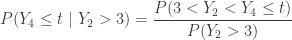
We now calculate the second probability in Example 3.
First calculate  . The probability
  is the probability of having at least 1 sample item less than
  , which is the complement of the probability of all sample items greater than .
The event  can occur in 16256 ways. Out of these many ways, 6972 of these satisfy the event . Thus we have:
Example 4
Draw a random sample  from the uniform distribution . The resulting order statistics are
  . Consider the conditional random variable
  . For this conditional distribution, find the following:
where  . Note that
  is the density function of .
Note that
In finding  , the range (0, 5) is broken up into 3 intervals (0, 3), (3, t) and (t, 5). The sample items fall into these intervals with probabilities
  ,
,  and
and  .
.
Since  , there is at most 1 sample item in the interval (0, 3). Since
  , there are at least 4 sample items in the interval (0, t). So the count in the interval (3, t) and the count in (0, 3) should add up to 4 or more items. The following shows all the cases for the event
  along with the corresponding multinomial probabilities.
After carrying the algebra and simplifying, we have the following:
For the event to happen, there is at most 1 sample item less than 3. So we have:
Then the conditional density is obtained by differentiating  .
.
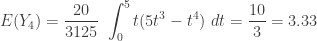
The following gives the conditional mean  .
.
To contrast, the following gives the information on the unconditional distribution of .
The unconditional mean of is about 3.33. With the additional information that , the average of is now 4.2. So a higher value of pulls up the mean of .
________________________________________________________________________
Practice problems
Practice problems to reinforce the calculation are found in the problem blog, a companion blog to this blog.
________________________________________________________________________


![\displaystyle \begin{aligned} p_k&=\frac{365}{365} \ \frac{364}{365} \ \frac{363}{365} \cdots \frac{365-(k-1)}{365} \\&=\frac{364}{365} \ \frac{363}{365} \cdots \frac{365-(k-1)}{365} \\&=\biggl[1-\frac{1}{365} \biggr] \ \biggl[1-\frac{2}{365} \biggr] \cdots \biggl[1-\frac{k-1}{365} \biggr] \ \ \ \ \ \ \ \ \ \ \ \ \ \ \ \ \ \ \ \ \ \ \ \ \ \ \ \ \ (1) \end{aligned}](https://s0.wp.com/latex.php?latex=%5Cdisplaystyle+%5Cbegin%7Baligned%7D+p_k%26%3D%5Cfrac%7B365%7D%7B365%7D+%5C+%5Cfrac%7B364%7D%7B365%7D+%5C+%5Cfrac%7B363%7D%7B365%7D+%5Ccdots+%5Cfrac%7B365-%28k-1%29%7D%7B365%7D+%5C%5C%26%3D%5Cfrac%7B364%7D%7B365%7D+%5C+%5Cfrac%7B363%7D%7B365%7D+%5Ccdots+%5Cfrac%7B365-%28k-1%29%7D%7B365%7D+%5C%5C%26%3D%5Cbiggl%5B1-%5Cfrac%7B1%7D%7B365%7D+%5Cbiggr%5D+%5C+%5Cbiggl%5B1-%5Cfrac%7B2%7D%7B365%7D+%5Cbiggr%5D+%5Ccdots+%5Cbiggl%5B1-%5Cfrac%7Bk-1%7D%7B365%7D+%5Cbiggr%5D+%5C+%5C+%5C+%5C+%5C+%5C+%5C+%5C+%5C+%5C+%5C+%5C+%5C+%5C+%5C+%5C+%5C+%5C+%5C+%5C+%5C+%5C+%5C+%5C+%5C+%5C+%5C+%5C+%5C+%281%29+%5Cend%7Baligned%7D&bg=ffffff&fg=333333&s=0&c=20201002)


![\displaystyle \begin{aligned} p_{n,k}&=\frac{n}{n} \ \frac{n-1}{n} \ \frac{n-2}{n} \cdots \frac{n-(k-1)}{n} \\&=\frac{n-1}{n} \ \frac{n-2}{n} \cdots \frac{n-(k-1)}{n} \\&=\biggl[1-\frac{1}{n} \biggr] \ \biggl[1-\frac{2}{n} \biggr] \cdots \biggl[1-\frac{k-1}{n} \biggr] \ \ \ \ \ \ \ \ \ \ \ \ \ \ \ \ \ \ \ \ \ \ \ \ \ \ \ \ \ (2) \end{aligned}](https://s0.wp.com/latex.php?latex=%5Cdisplaystyle+%5Cbegin%7Baligned%7D+p_%7Bn%2Ck%7D%26%3D%5Cfrac%7Bn%7D%7Bn%7D+%5C+%5Cfrac%7Bn-1%7D%7Bn%7D+%5C+%5Cfrac%7Bn-2%7D%7Bn%7D+%5Ccdots+%5Cfrac%7Bn-%28k-1%29%7D%7Bn%7D+%5C%5C%26%3D%5Cfrac%7Bn-1%7D%7Bn%7D+%5C+%5Cfrac%7Bn-2%7D%7Bn%7D+%5Ccdots+%5Cfrac%7Bn-%28k-1%29%7D%7Bn%7D+%5C%5C%26%3D%5Cbiggl%5B1-%5Cfrac%7B1%7D%7Bn%7D+%5Cbiggr%5D+%5C+%5Cbiggl%5B1-%5Cfrac%7B2%7D%7Bn%7D+%5Cbiggr%5D+%5Ccdots+%5Cbiggl%5B1-%5Cfrac%7Bk-1%7D%7Bn%7D+%5Cbiggr%5D+%5C+%5C+%5C+%5C+%5C+%5C+%5C+%5C+%5C+%5C+%5C+%5C+%5C+%5C+%5C+%5C+%5C+%5C+%5C+%5C+%5C+%5C+%5C+%5C+%5C+%5C+%5C+%5C+%5C+%282%29+%5Cend%7Baligned%7D&bg=ffffff&fg=333333&s=0&c=20201002)

![P[X_6=k]](https://s0.wp.com/latex.php?latex=P%5BX_6%3Dk%5D&bg=ffffff&fg=333333&s=0&c=20201002)


![P[X_n=k]](https://s0.wp.com/latex.php?latex=P%5BX_n%3Dk%5D&bg=ffffff&fg=333333&s=0&c=20201002)
![\displaystyle \begin{aligned} P[X_n=k]&=\frac{n}{n} \times \frac{n-1}{n} \times \cdots \times \frac{n-(k-2)}{n} \times \frac{k-1}{n} \\&=\frac{n-1}{n} \times \cdots \times \frac{n-(k-2)}{n} \times \frac{k-1}{n} \\&=\frac{(n-1) \times (n-2) \times \cdots \times (n-(k-2)) \times (k-1)}{n^{k-1}} \\&=\biggl[1-\frac{1}{n} \biggr] \times \biggl[1-\frac{2}{n} \biggr] \times \cdots \times \biggl[1-\frac{k-2}{n}\biggr] \times \frac{k-1}{n} \ \ \ \ \ \ \ (3) \end{aligned}](https://s0.wp.com/latex.php?latex=%5Cdisplaystyle+%5Cbegin%7Baligned%7D+P%5BX_n%3Dk%5D%26%3D%5Cfrac%7Bn%7D%7Bn%7D+%5Ctimes+%5Cfrac%7Bn-1%7D%7Bn%7D+%5Ctimes+%5Ccdots+%5Ctimes+%5Cfrac%7Bn-%28k-2%29%7D%7Bn%7D+%5Ctimes+%5Cfrac%7Bk-1%7D%7Bn%7D+%5C%5C%26%3D%5Cfrac%7Bn-1%7D%7Bn%7D+%5Ctimes+%5Ccdots+%5Ctimes+%5Cfrac%7Bn-%28k-2%29%7D%7Bn%7D+%5Ctimes+%5Cfrac%7Bk-1%7D%7Bn%7D+%5C%5C%26%3D%5Cfrac%7B%28n-1%29+%5Ctimes+%28n-2%29+%5Ctimes+%5Ccdots+%5Ctimes+%28n-%28k-2%29%29+%5Ctimes+%28k-1%29%7D%7Bn%5E%7Bk-1%7D%7D+%5C%5C%26%3D%5Cbiggl%5B1-%5Cfrac%7B1%7D%7Bn%7D+%5Cbiggr%5D+%5Ctimes+%5Cbiggl%5B1-%5Cfrac%7B2%7D%7Bn%7D+%5Cbiggr%5D+%5Ctimes+%5Ccdots+%5Ctimes+%5Cbiggl%5B1-%5Cfrac%7Bk-2%7D%7Bn%7D%5Cbiggr%5D+%5Ctimes+%5Cfrac%7Bk-1%7D%7Bn%7D++%5C+%5C+%5C+%5C+%5C+%5C+%5C+%283%29+%5Cend%7Baligned%7D&bg=ffffff&fg=333333&s=0&c=20201002)


![E[X_n]](https://s0.wp.com/latex.php?latex=E%5BX_n%5D&bg=ffffff&fg=333333&s=0&c=20201002)
![E[X_{365}]=24.62](https://s0.wp.com/latex.php?latex=E%5BX_%7B365%7D%5D%3D24.62&bg=ffffff&fg=333333&s=0&c=20201002)
![P[X_n>k]](https://s0.wp.com/latex.php?latex=P%5BX_n%3Ek%5D&bg=ffffff&fg=333333&s=0&c=20201002)
![P[X_n \le k]](https://s0.wp.com/latex.php?latex=P%5BX_n+%5Cle+k%5D&bg=ffffff&fg=333333&s=0&c=20201002)

![\displaystyle P[X_n>k]=\biggl[1-\frac{1}{n} \biggr] \ \biggl[1-\frac{2}{n} \biggr] \cdots \biggl[1-\frac{k-1}{n} \biggr] \ \ \ \ \ \ \ \ \ \ \ \ \ \ \ \ \ \ \ \ \ \ \ \ (4)](https://s0.wp.com/latex.php?latex=%5Cdisplaystyle+P%5BX_n%3Ek%5D%3D%5Cbiggl%5B1-%5Cfrac%7B1%7D%7Bn%7D+%5Cbiggr%5D+%5C+%5Cbiggl%5B1-%5Cfrac%7B2%7D%7Bn%7D+%5Cbiggr%5D+%5Ccdots+%5Cbiggl%5B1-%5Cfrac%7Bk-1%7D%7Bn%7D+%5Cbiggr%5D+%5C+%5C+%5C+%5C+%5C+%5C+%5C+%5C+%5C+%5C+%5C+%5C+%5C+%5C+%5C+%5C+%5C+%5C+%5C+%5C+%5C+%5C+%5C+%5C+%284%29&bg=ffffff&fg=333333&s=0&c=20201002)

![P[X_{365} \le k]](https://s0.wp.com/latex.php?latex=P%5BX_%7B365%7D+%5Cle+k%5D&bg=ffffff&fg=333333&s=0&c=20201002)
![P[X_{365}>k]](https://s0.wp.com/latex.php?latex=P%5BX_%7B365%7D%3Ek%5D&bg=ffffff&fg=333333&s=0&c=20201002)


![\begin{array}{ccccccc} k & \text{ } & P[X_{365}>k] & \text{ } & P[X_{365} \le k] & \text{ } & \text{Percentile} \\ \text{ } & \text{ } & \text{ } & \text{ } & \text{ } & \\ 14 & \text{ } & 0.77690 & & 0.22310 & \\ 15 & \text{ } & 0.74710 & & 0.25290 & \text{ } & \text{25th Percentile} \\ 16 & \text{ } & 0.71640 & & 0.28360 & \\ \text{ } & \text{ } & \text{ } & \text{ } & \text{ } & \\ 22 & \text{ } & 0.52430 & & 0.47570 & \\ 23 & \text{ } & 0.49270 & & 0.50730 & \text{ } & \text{50th Percentile} \\ 24 & \text{ } & 0.46166 & & 0.53834 & \\ \text{ } & \text{ } & \text{ } & \text{ } & \text{ } & \\ 31 & \text{ } & 0.26955 & & 0.73045 & \\ 32 & \text{ } & 0.24665 & & 0.75335 & \text{ } & \text{75th Percentile} \\ 33 & \text{ } & 0.22503 & & 0.77497 & \\ \text{ } & \text{ } & \text{ } & \text{ } & \text{ } & \\ 40 & \text{ } & 0.10877 & & 0.89123 & \\ 41 & \text{ } & 0.09685 & & 0.90315 & \text{ } & \text{90th Percentile} \\ 42 & \text{ } & 0.08597 & & 0.91403 & \\ \text{ } & \text{ } & \text{ } & \text{ } & \text{ } & \\ 46 & \text{ } & 0.05175 & & 0.94825 & \\ 47 & \text{ } & 0.04523 & & 0.95477 & \text{ } & \text{95th Percentile} \\ 48 & \text{ } & 0.03940 & & 0.96060 & \\ \text{ } & \text{ } & \text{ } & \text{ } & \text{ } & \\ 56 & \text{ } & 0.01167 & & 0.98833 & \\ 57 & \text{ } & 0.00988 & & 0.99012 & \text{ } & \text{99th Percentile} \\ 58 & \text{ } & 0.00834 & & 0.99166 & \\ \end{array}](https://s0.wp.com/latex.php?latex=%5Cbegin%7Barray%7D%7Bccccccc%7D++++k+%26++%5Ctext%7B+%7D+%26+P%5BX_%7B365%7D%3Ek%5D++%26+%5Ctext%7B+%7D+%26+P%5BX_%7B365%7D+%5Cle+k%5D+%26+%5Ctext%7B+%7D+%26+%5Ctext%7BPercentile%7D+%5C%5C++++%5Ctext%7B+%7D+%26+++%5Ctext%7B+%7D+%26+%5Ctext%7B+%7D+%26+%5Ctext%7B+%7D+%26+%5Ctext%7B+%7D+%26++%5C%5C+++14+%26+++%5Ctext%7B+%7D+%26+0.77690+%26++%26+0.22310+%26++%5C%5C+++15+%26+++%5Ctext%7B+%7D+%26+0.74710+%26++%26+0.25290+%26+%5Ctext%7B+%7D+%26+%5Ctext%7B25th+Percentile%7D+%5C%5C+++16+%26+++%5Ctext%7B+%7D+%26+0.71640+%26++%26+0.28360+%26++%5C%5C++%5Ctext%7B+%7D+%26+++%5Ctext%7B+%7D+%26+%5Ctext%7B+%7D+%26+%5Ctext%7B+%7D+%26+%5Ctext%7B+%7D+%26++%5C%5C+++22+%26+++%5Ctext%7B+%7D+%26+0.52430+%26++%26+0.47570+%26++%5C%5C+++23+%26+++%5Ctext%7B+%7D+%26+0.49270+%26++%26+0.50730+%26+%5Ctext%7B+%7D+%26+%5Ctext%7B50th+Percentile%7D++%5C%5C+++24+%26+++%5Ctext%7B+%7D+%26+0.46166+%26++%26+0.53834+%26++%5C%5C++%5Ctext%7B+%7D+%26+++%5Ctext%7B+%7D+%26+%5Ctext%7B+%7D+%26+%5Ctext%7B+%7D+%26+%5Ctext%7B+%7D+%26++%5C%5C+++31+%26+++%5Ctext%7B+%7D+%26+0.26955+%26++%26+0.73045+%26++%5C%5C+++32+%26+++%5Ctext%7B+%7D+%26+0.24665+%26++%26+0.75335+%26+%5Ctext%7B+%7D+%26+%5Ctext%7B75th+Percentile%7D+%5C%5C+++++++++33+%26+++%5Ctext%7B+%7D+%26+0.22503+%26++%26+0.77497+%26++%5C%5C++%5Ctext%7B+%7D+%26+++%5Ctext%7B+%7D+%26+%5Ctext%7B+%7D+%26+%5Ctext%7B+%7D+%26+%5Ctext%7B+%7D+%26++%5C%5C+++40+%26+++%5Ctext%7B+%7D+%26+0.10877+%26++%26+0.89123+%26++%5C%5C+++41+%26+++%5Ctext%7B+%7D+%26+0.09685+%26++%26+0.90315+%26+%5Ctext%7B+%7D+%26+%5Ctext%7B90th+Percentile%7D+%5C%5C+++42+%26+++%5Ctext%7B+%7D+%26+0.08597+%26++%26+0.91403+%26++%5C%5C++%5Ctext%7B+%7D+%26+++%5Ctext%7B+%7D+%26+%5Ctext%7B+%7D+%26+%5Ctext%7B+%7D+%26+%5Ctext%7B+%7D+%26++%5C%5C+++46+%26+++%5Ctext%7B+%7D+%26+0.05175+%26++%26+0.94825+%26++%5C%5C+++47+%26+++%5Ctext%7B+%7D+%26+0.04523+%26++%26+0.95477+%26+%5Ctext%7B+%7D+%26+%5Ctext%7B95th+Percentile%7D+%5C%5C++++48+%26++%5Ctext%7B+%7D+%26+0.03940+%26++%26+0.96060+%26++%5C%5C++%5Ctext%7B+%7D+%26+++%5Ctext%7B+%7D+%26+%5Ctext%7B+%7D+%26+%5Ctext%7B+%7D+%26+%5Ctext%7B+%7D+%26++%5C%5C++++56+%26++%5Ctext%7B+%7D+%26+0.01167+%26++%26+0.98833+%26++%5C%5C++57+%26++%5Ctext%7B+%7D+%26+0.00988+%26++%26+0.99012+%26+%5Ctext%7B+%7D+%26+%5Ctext%7B99th+Percentile%7D+%5C%5C++58+%26++%5Ctext%7B+%7D+%26+0.00834+%26++%26+0.99166+%26++%5C%5C++++++%5Cend%7Barray%7D&bg=ffffff&fg=333333&s=0&c=20201002)

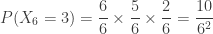
 possibilities. This number is 67,108,864. So 2 raised to 26 is a little over 67 millions. So the password given by John is not just one password, but is a generic one with over 67 million possibilities. There is a one in 67 million chance in correctly guessing the correct password if John chooses the upper case letters randomly. This is much better odds than winning the Powerball lottery, one in 292,201,338, which one in 292 million. But it is still an undeniably strong password.
 . Sometimes the notations
  ,
,  and
and  are used. Regardless of the notation, the calculation is
 is the product of all the positive integers up to and including
  ,
,  ,
,  ,
,  . To make the formula work correctly, we make
  .
.


![\displaystyle \begin{array}{rrr} k &\text{ } & P[X=k] \\ \text{ } & \text{ } & \text{ } \\ 0 &\text{ } & 0.00000001 \\ 1 &\text{ } & 0.00000039 \\ 2 &\text{ } & 0.00000484 \\ 3 &\text{ } & 0.00003874 \\ 4 &\text{ } & 0.00022277 \\ 5 &\text{ } & 0.00098020 \\ 6 &\text{ } & 0.00343069 \\ 7 &\text{ } & 0.00980198 \\ 8 &\text{ } & 0.02327971 \\ 9 &\text{ } & 0.04655942 \\ 10 &\text{ } & 0.07915102 \\ 11 &\text{ } & 0.11512876 \\ 12 &\text{ } & 0.14391094 \\ 13 &\text{ } & 0.15498102 \\ 14 &\text{ } & 0.14391094 \\ 15 &\text{ } & 0.11512876 \\ 16 &\text{ } & 0.07915102 \\ 17 &\text{ } & 0.04655942 \\ 18 &\text{ } & 0.02327971 \\ 19 &\text{ } & 0.00980198 \\ 20 &\text{ } & 0.00343069 \\ 21 &\text{ } & 0.00098020 \\ 22 &\text{ } & 0.00022277 \\ 23 &\text{ } & 0.00003874 \\ 24 &\text{ } & 0.00000484 \\ 25 &\text{ } & 0.00000039 \\ 26 &\text{ } & 0.00000001 \\ \end{array}](https://s0.wp.com/latex.php?latex=%5Cdisplaystyle+%5Cbegin%7Barray%7D%7Brrr%7D+k+%26%5Ctext%7B+%7D+%26+P%5BX%3Dk%5D++%5C%5C++%5Ctext%7B+%7D+%26+%5Ctext%7B+%7D+%26+%5Ctext%7B+%7D++%5C%5C++0+%26%5Ctext%7B+%7D+%26+0.00000001++%5C%5C+++++1+%26%5Ctext%7B+%7D+%26+0.00000039+++%5C%5C++2+%26%5Ctext%7B+%7D+%26+0.00000484+++%5C%5C++3+%26%5Ctext%7B+%7D+%26+0.00003874+++%5C%5C++4+%26%5Ctext%7B+%7D+%26+0.00022277+++%5C%5C++5+%26%5Ctext%7B+%7D+%26+0.00098020+++%5C%5C++6+%26%5Ctext%7B+%7D+%26+0.00343069+++%5C%5C++7+%26%5Ctext%7B+%7D+%26+0.00980198+++%5C%5C++8+%26%5Ctext%7B+%7D+%26+0.02327971+++%5C%5C++9+%26%5Ctext%7B+%7D+%26+0.04655942+++%5C%5C++10+%26%5Ctext%7B+%7D+%26+0.07915102+++%5C%5C++11+%26%5Ctext%7B+%7D+%26+0.11512876+++%5C%5C++12+%26%5Ctext%7B+%7D+%26+0.14391094+++%5C%5C++13+%26%5Ctext%7B+%7D+%26+0.15498102+++%5C%5C++14+%26%5Ctext%7B+%7D+%26+0.14391094+++%5C%5C++15+%26%5Ctext%7B+%7D+%26+0.11512876+++%5C%5C++16+%26%5Ctext%7B+%7D+%26+0.07915102+++%5C%5C++17+%26%5Ctext%7B+%7D+%26+0.04655942+++%5C%5C++18+%26%5Ctext%7B+%7D+%26+0.02327971+++%5C%5C++19+%26%5Ctext%7B+%7D+%26+0.00980198+++%5C%5C++20+%26%5Ctext%7B+%7D+%26+0.00343069+++%5C%5C++21+%26%5Ctext%7B+%7D+%26+0.00098020+++%5C%5C++22+%26%5Ctext%7B+%7D+%26+0.00022277+++%5C%5C++23+%26%5Ctext%7B+%7D+%26+0.00003874+++%5C%5C++24+%26%5Ctext%7B+%7D+%26+0.00000484+++%5C%5C++25+%26%5Ctext%7B+%7D+%26+0.00000039+++%5C%5C++26+%26%5Ctext%7B+%7D+%26+0.00000001+++%5C%5C++%5Cend%7Barray%7D&bg=ffffff&fg=333333&s=0&c=20201002)
 where
where  add up to 67.3% of the 67,108,864 possibilities.
 be the number of upper case letters in the 26-character password. Then the random variable
  (26 Bernoulli trials) and the probability of success
  in each trial, which is the probability that a character is upper case, assuming that he determines the upper/lower case by a coin toss. The following is the probability function:
![\displaystyle P(X=x)=\binom{26}{x} \biggl[\frac{1}{2}\biggr]^x \biggl[\frac{1}{2}\biggr]^{26-x}=\binom{26}{x} \biggl[\frac{1}{2}\biggr]^{26}](https://s0.wp.com/latex.php?latex=%5Cdisplaystyle+P%28X%3Dx%29%3D%5Cbinom%7B26%7D%7Bx%7D+%5Cbiggl%5B%5Cfrac%7B1%7D%7B2%7D%5Cbiggr%5D%5Ex+%5Cbiggl%5B%5Cfrac%7B1%7D%7B2%7D%5Cbiggr%5D%5E%7B26-x%7D%3D%5Cbinom%7B26%7D%7Bx%7D+%5Cbiggl%5B%5Cfrac%7B1%7D%7B2%7D%5Cbiggr%5D%5E%7B26%7D&bg=ffffff&fg=333333&s=0&c=20201002)
 . The quantity
  is the probability that the number of upper case letters is
  . Here,
  is the number of ways to choose

 and the probability of the other outcome (called failure) is
  . The random variable
  gives the likelihood of achieving
  (assuming that the random variable
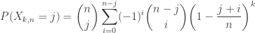
![\displaystyle P(Y_j \le t)=\sum \limits_{k=j}^n \binom{n}{k} \ \biggl[ F(t) \biggr]^k \ \biggl[1-F(x) \biggr]^{n-k} \ \ \ \ \ \ \ \ \ \ \ \ \ \ (1)](https://s0.wp.com/latex.php?latex=%5Cdisplaystyle+P%28Y_j+%5Cle+t%29%3D%5Csum+%5Climits_%7Bk%3Dj%7D%5En+%5Cbinom%7Bn%7D%7Bk%7D+%5C+%5Cbiggl%5B+F%28t%29+%5Cbiggr%5D%5Ek+%5C+%5Cbiggl%5B1-F%28x%29+%5Cbiggr%5D%5E%7Bn-k%7D+%5C+%5C+%5C+%5C+%5C+%5C+%5C+%5C+%5C+%5C+%5C+%5C+%5C+%5C+%281%29&bg=ffffff&fg=333333&s=0&c=20201002)
![\displaystyle P(Y_j > t)=\sum \limits_{k=0}^{j-1} \binom{n}{k} \ \biggl[ F(t) \biggr]^k \ \biggl[1-F(x) \biggr]^{n-k} \ \ \ \ \ \ \ \ \ \ \ \ \ \ (2)](https://s0.wp.com/latex.php?latex=%5Cdisplaystyle+P%28Y_j+%3E+t%29%3D%5Csum+%5Climits_%7Bk%3D0%7D%5E%7Bj-1%7D+%5Cbinom%7Bn%7D%7Bk%7D+%5C+%5Cbiggl%5B+F%28t%29+%5Cbiggr%5D%5Ek+%5C+%5Cbiggl%5B1-F%28x%29+%5Cbiggr%5D%5E%7Bn-k%7D+%5C+%5C+%5C+%5C+%5C+%5C+%5C+%5C+%5C+%5C+%5C+%5C+%5C+%5C+%282%29&bg=ffffff&fg=333333&s=0&c=20201002)


![\displaystyle \begin{aligned} P(Y_4<2<Y_5<Y_6<3<Y_7)&=\frac{10!}{4! \ 2! \ 4!} \biggl[\frac{2}{4} \biggr]^4 \ \biggl[\frac{1}{4} \biggr]^2 \ \biggl[\frac{1}{4} \biggr]^4 \\&\text{ } \\&=\frac{50400}{1048567} \\&\text{ } \\&=0.0481 \end{aligned}](https://s0.wp.com/latex.php?latex=%5Cdisplaystyle+%5Cbegin%7Baligned%7D+P%28Y_4%3C2%3CY_5%3CY_6%3C3%3CY_7%29%26%3D%5Cfrac%7B10%21%7D%7B4%21+%5C+2%21+%5C+4%21%7D+%5Cbiggl%5B%5Cfrac%7B2%7D%7B4%7D+%5Cbiggr%5D%5E4+%5C+%5Cbiggl%5B%5Cfrac%7B1%7D%7B4%7D+%5Cbiggr%5D%5E2+%5C+%5Cbiggl%5B%5Cfrac%7B1%7D%7B4%7D+%5Cbiggr%5D%5E4+%5C%5C%26%5Ctext%7B+%7D+%5C%5C%26%3D%5Cfrac%7B50400%7D%7B1048567%7D+%5C%5C%26%5Ctext%7B+%7D+%5C%5C%26%3D0.0481++%5Cend%7Baligned%7D&bg=ffffff&fg=333333&s=0&c=20201002)
![\displaystyle \begin{aligned} P(Y_4<2<Y_6<3<Y_7)&=\frac{10!}{4! \ 2! \ 4!} \biggl[\frac{2}{4} \biggr]^4 \ \biggl[\frac{1}{4} \biggr]^2 \ \biggl[\frac{1}{4} \biggr]^4 \\& \ \ \ \ + \frac{10!}{5! \ 1! \ 4!} \biggl[\frac{2}{4} \biggr]^5 \ \biggl[\frac{1}{4} \biggr]^1 \ \biggl[\frac{1}{4} \biggr]^4 \\&\text{ } \\&=\frac{50400+40320}{1048567} \\&\text{ } \\&=\frac{90720}{1048567} \\&\text{ } \\&=0.0865 \end{aligned}](https://s0.wp.com/latex.php?latex=%5Cdisplaystyle+%5Cbegin%7Baligned%7D+P%28Y_4%3C2%3CY_6%3C3%3CY_7%29%26%3D%5Cfrac%7B10%21%7D%7B4%21+%5C+2%21+%5C+4%21%7D+%5Cbiggl%5B%5Cfrac%7B2%7D%7B4%7D+%5Cbiggr%5D%5E4+%5C+%5Cbiggl%5B%5Cfrac%7B1%7D%7B4%7D+%5Cbiggr%5D%5E2+%5C+%5Cbiggl%5B%5Cfrac%7B1%7D%7B4%7D+%5Cbiggr%5D%5E4+%5C%5C%26+%5C+%5C+%5C+%5C+%2B+%5Cfrac%7B10%21%7D%7B5%21+%5C+1%21+%5C+4%21%7D+%5Cbiggl%5B%5Cfrac%7B2%7D%7B4%7D+%5Cbiggr%5D%5E5+%5C+%5Cbiggl%5B%5Cfrac%7B1%7D%7B4%7D+%5Cbiggr%5D%5E1+%5C+%5Cbiggl%5B%5Cfrac%7B1%7D%7B4%7D+%5Cbiggr%5D%5E4+%5C%5C%26%5Ctext%7B+%7D+%5C%5C%26%3D%5Cfrac%7B50400%2B40320%7D%7B1048567%7D+%5C%5C%26%5Ctext%7B+%7D+%5C%5C%26%3D%5Cfrac%7B90720%7D%7B1048567%7D+%5C%5C%26%5Ctext%7B+%7D+%5C%5C%26%3D0.0865++%5Cend%7Baligned%7D&bg=ffffff&fg=333333&s=0&c=20201002)
![\displaystyle \begin{aligned} \frac{6!}{a! \ b! \ c!} \ \biggl[\frac{1}{4} \biggr]^a \ \biggl[\frac{2}{4} \biggr]^b \ \biggl[\frac{1}{4} \biggr]^c&=\frac{6!}{0! \ 4! \ 2!} \ \biggl[\frac{1}{4} \biggr]^0 \ \biggl[\frac{2}{4} \biggr]^4 \ \biggl[\frac{1}{4} \biggr]^2=\frac{240}{4096} \\&\text{ } \\&=\frac{6!}{0! \ 5! \ 1!} \ \biggl[\frac{1}{4} \biggr]^0 \ \biggl[\frac{2}{4} \biggr]^5 \ \biggl[\frac{1}{4} \biggr]^1=\frac{192}{4096} \\&\text{ } \\&=\frac{6!}{0! \ 6! \ 0!} \ \biggl[\frac{1}{4} \biggr]^0 \ \biggl[\frac{2}{4} \biggr]^6 \ \biggl[\frac{1}{4} \biggr]^0=\frac{64}{4096} \\&\text{ } \\&=\frac{6!}{1! \ 3! \ 2!} \ \biggl[\frac{1}{4} \biggr]^1 \ \biggl[\frac{2}{4} \biggr]^3 \ \biggl[\frac{1}{4} \biggr]^2=\frac{480}{4096} \\&\text{ } \\&=\frac{6!}{1! \ 4! \ 1!} \ \biggl[\frac{1}{4} \biggr]^1 \ \biggl[\frac{2}{4} \biggr]^4 \ \biggl[\frac{1}{4} \biggr]^1=\frac{480}{4096} \\&\text{ } \\&=\frac{6!}{1! \ 5! \ 0!} \ \biggl[\frac{1}{4} \biggr]^1 \ \biggl[\frac{2}{4} \biggr]^5 \ \biggl[\frac{1}{4} \biggr]^0=\frac{192}{4096} \\&\text{ } \\&=\text{sum of probabilities }=\frac{1648}{4096}=0.4023\end{aligned}](https://s0.wp.com/latex.php?latex=%5Cdisplaystyle+%5Cbegin%7Baligned%7D+%5Cfrac%7B6%21%7D%7Ba%21+%5C+b%21+%5C+c%21%7D+%5C+%5Cbiggl%5B%5Cfrac%7B1%7D%7B4%7D+%5Cbiggr%5D%5Ea+%5C+%5Cbiggl%5B%5Cfrac%7B2%7D%7B4%7D+%5Cbiggr%5D%5Eb+%5C+%5Cbiggl%5B%5Cfrac%7B1%7D%7B4%7D+%5Cbiggr%5D%5Ec%26%3D%5Cfrac%7B6%21%7D%7B0%21+%5C+4%21+%5C+2%21%7D+%5C+%5Cbiggl%5B%5Cfrac%7B1%7D%7B4%7D+%5Cbiggr%5D%5E0+%5C+%5Cbiggl%5B%5Cfrac%7B2%7D%7B4%7D+%5Cbiggr%5D%5E4+%5C+%5Cbiggl%5B%5Cfrac%7B1%7D%7B4%7D+%5Cbiggr%5D%5E2%3D%5Cfrac%7B240%7D%7B4096%7D+%5C%5C%26%5Ctext%7B+%7D+%5C%5C%26%3D%5Cfrac%7B6%21%7D%7B0%21+%5C+5%21+%5C+1%21%7D+%5C+%5Cbiggl%5B%5Cfrac%7B1%7D%7B4%7D+%5Cbiggr%5D%5E0+%5C+%5Cbiggl%5B%5Cfrac%7B2%7D%7B4%7D+%5Cbiggr%5D%5E5+%5C+%5Cbiggl%5B%5Cfrac%7B1%7D%7B4%7D+%5Cbiggr%5D%5E1%3D%5Cfrac%7B192%7D%7B4096%7D+%5C%5C%26%5Ctext%7B+%7D+%5C%5C%26%3D%5Cfrac%7B6%21%7D%7B0%21+%5C+6%21+%5C+0%21%7D+%5C+%5Cbiggl%5B%5Cfrac%7B1%7D%7B4%7D+%5Cbiggr%5D%5E0+%5C+%5Cbiggl%5B%5Cfrac%7B2%7D%7B4%7D+%5Cbiggr%5D%5E6+%5C+%5Cbiggl%5B%5Cfrac%7B1%7D%7B4%7D+%5Cbiggr%5D%5E0%3D%5Cfrac%7B64%7D%7B4096%7D+%5C%5C%26%5Ctext%7B+%7D+%5C%5C%26%3D%5Cfrac%7B6%21%7D%7B1%21+%5C+3%21+%5C+2%21%7D+%5C+%5Cbiggl%5B%5Cfrac%7B1%7D%7B4%7D+%5Cbiggr%5D%5E1+%5C+%5Cbiggl%5B%5Cfrac%7B2%7D%7B4%7D+%5Cbiggr%5D%5E3+%5C+%5Cbiggl%5B%5Cfrac%7B1%7D%7B4%7D+%5Cbiggr%5D%5E2%3D%5Cfrac%7B480%7D%7B4096%7D+%5C%5C%26%5Ctext%7B+%7D+%5C%5C%26%3D%5Cfrac%7B6%21%7D%7B1%21+%5C+4%21+%5C+1%21%7D+%5C+%5Cbiggl%5B%5Cfrac%7B1%7D%7B4%7D+%5Cbiggr%5D%5E1+%5C+%5Cbiggl%5B%5Cfrac%7B2%7D%7B4%7D+%5Cbiggr%5D%5E4+%5C+%5Cbiggl%5B%5Cfrac%7B1%7D%7B4%7D+%5Cbiggr%5D%5E1%3D%5Cfrac%7B480%7D%7B4096%7D+%5C%5C%26%5Ctext%7B+%7D+%5C%5C%26%3D%5Cfrac%7B6%21%7D%7B1%21+%5C+5%21+%5C+0%21%7D+%5C+%5Cbiggl%5B%5Cfrac%7B1%7D%7B4%7D+%5Cbiggr%5D%5E1+%5C+%5Cbiggl%5B%5Cfrac%7B2%7D%7B4%7D+%5Cbiggr%5D%5E5+%5C+%5Cbiggl%5B%5Cfrac%7B1%7D%7B4%7D+%5Cbiggr%5D%5E0%3D%5Cfrac%7B192%7D%7B4096%7D+%5C%5C%26%5Ctext%7B+%7D+%5C%5C%26%3D%5Ctext%7Bsum+of+probabilities+%7D%3D%5Cfrac%7B1648%7D%7B4096%7D%3D0.4023%5Cend%7Baligned%7D&bg=ffffff&fg=333333&s=0&c=20201002)


![\displaystyle [0, 1, 3, 3] \ \ \ \ \ \ \frac{280}{78125}=\frac{7!}{0! \ 1! \ 3! \ 3!} \ \biggl[\frac{1}{5} \biggr]^0 \ \biggl[\frac{2}{5} \biggr]^1 \ \biggl[\frac{1}{5} \biggr]^3 \ \biggl[\frac{1}{5} \biggr]^3](https://s0.wp.com/latex.php?latex=%5Cdisplaystyle+%5B0%2C+1%2C+3%2C+3%5D+%5C+%5C+%5C+%5C+%5C+%5C+%5Cfrac%7B280%7D%7B78125%7D%3D%5Cfrac%7B7%21%7D%7B0%21+%5C+1%21+%5C+3%21+%5C+3%21%7D+%5C+%5Cbiggl%5B%5Cfrac%7B1%7D%7B5%7D+%5Cbiggr%5D%5E0+%5C+%5Cbiggl%5B%5Cfrac%7B2%7D%7B5%7D+%5Cbiggr%5D%5E1+%5C+%5Cbiggl%5B%5Cfrac%7B1%7D%7B5%7D+%5Cbiggr%5D%5E3+%5C+%5Cbiggl%5B%5Cfrac%7B1%7D%7B5%7D+%5Cbiggr%5D%5E3&bg=ffffff&fg=333333&s=0&c=20201002)
![\displaystyle [0, 1, 4, 2] \ \ \ \ \ \ \frac{210}{78125}](https://s0.wp.com/latex.php?latex=%5Cdisplaystyle+%5B0%2C+1%2C+4%2C+2%5D+%5C+%5C+%5C+%5C+%5C+%5C+%5Cfrac%7B210%7D%7B78125%7D&bg=ffffff&fg=333333&s=0&c=20201002)
![\displaystyle [0, 1, 5, 1] \ \ \ \ \ \ \frac{84}{78125}](https://s0.wp.com/latex.php?latex=%5Cdisplaystyle+%5B0%2C+1%2C+5%2C+1%5D+%5C+%5C+%5C+%5C+%5C+%5C+%5Cfrac%7B84%7D%7B78125%7D&bg=ffffff&fg=333333&s=0&c=20201002)
![\displaystyle [0, 1, 6, 0] \ \ \ \ \ \ \frac{14}{78125}](https://s0.wp.com/latex.php?latex=%5Cdisplaystyle+%5B0%2C+1%2C+6%2C+0%5D+%5C+%5C+%5C+%5C+%5C+%5C+%5Cfrac%7B14%7D%7B78125%7D&bg=ffffff&fg=333333&s=0&c=20201002)
![\displaystyle [0, 2, 2, 3] \ \ \ \ \ \ \frac{840}{78125}](https://s0.wp.com/latex.php?latex=%5Cdisplaystyle+%5B0%2C+2%2C+2%2C+3%5D+%5C+%5C+%5C+%5C+%5C+%5C+%5Cfrac%7B840%7D%7B78125%7D&bg=ffffff&fg=333333&s=0&c=20201002)
![\displaystyle [0, 2, 3, 2] \ \ \ \ \ \ \frac{840}{78125}](https://s0.wp.com/latex.php?latex=%5Cdisplaystyle+%5B0%2C+2%2C+3%2C+2%5D+%5C+%5C+%5C+%5C+%5C+%5C+%5Cfrac%7B840%7D%7B78125%7D&bg=ffffff&fg=333333&s=0&c=20201002)
![\displaystyle [0, 2, 4, 1] \ \ \ \ \ \ \frac{420}{78125}](https://s0.wp.com/latex.php?latex=%5Cdisplaystyle+%5B0%2C+2%2C+4%2C+1%5D+%5C+%5C+%5C+%5C+%5C+%5C+%5Cfrac%7B420%7D%7B78125%7D&bg=ffffff&fg=333333&s=0&c=20201002)
![\displaystyle [0, 2, 5, 0] \ \ \ \ \ \ \frac{84}{78125}](https://s0.wp.com/latex.php?latex=%5Cdisplaystyle+%5B0%2C+2%2C+5%2C+0%5D+%5C+%5C+%5C+%5C+%5C+%5C+%5Cfrac%7B84%7D%7B78125%7D&bg=ffffff&fg=333333&s=0&c=20201002)
![\displaystyle [0, 3, 1, 3] \ \ \ \ \ \ \frac{1120}{78125}=\frac{7!}{0! \ 3! \ 1! \ 3!} \ \biggl[\frac{1}{5} \biggr]^0 \ \biggl[\frac{2}{5} \biggr]^3 \ \biggl[\frac{1}{5} \biggr]^1 \ \biggl[\frac{1}{5} \biggr]^3](https://s0.wp.com/latex.php?latex=%5Cdisplaystyle+%5B0%2C+3%2C+1%2C+3%5D+%5C+%5C+%5C+%5C+%5C+%5C+%5Cfrac%7B1120%7D%7B78125%7D%3D%5Cfrac%7B7%21%7D%7B0%21+%5C+3%21+%5C+1%21+%5C+3%21%7D+%5C+%5Cbiggl%5B%5Cfrac%7B1%7D%7B5%7D+%5Cbiggr%5D%5E0+%5C+%5Cbiggl%5B%5Cfrac%7B2%7D%7B5%7D+%5Cbiggr%5D%5E3+%5C+%5Cbiggl%5B%5Cfrac%7B1%7D%7B5%7D+%5Cbiggr%5D%5E1+%5C+%5Cbiggl%5B%5Cfrac%7B1%7D%7B5%7D+%5Cbiggr%5D%5E3&bg=ffffff&fg=333333&s=0&c=20201002)
![\displaystyle [0, 3, 2, 2] \ \ \ \ \ \ \frac{1680}{78125}](https://s0.wp.com/latex.php?latex=%5Cdisplaystyle+%5B0%2C+3%2C+2%2C+2%5D+%5C+%5C+%5C+%5C+%5C+%5C+%5Cfrac%7B1680%7D%7B78125%7D&bg=ffffff&fg=333333&s=0&c=20201002)
![\displaystyle [0, 3, 3, 1] \ \ \ \ \ \ \frac{1120}{78125}](https://s0.wp.com/latex.php?latex=%5Cdisplaystyle+%5B0%2C+3%2C+3%2C+1%5D+%5C+%5C+%5C+%5C+%5C+%5C+%5Cfrac%7B1120%7D%7B78125%7D&bg=ffffff&fg=333333&s=0&c=20201002)
![\displaystyle [0, 3, 4, 0] \ \ \ \ \ \ \frac{280}{78125}](https://s0.wp.com/latex.php?latex=%5Cdisplaystyle+%5B0%2C+3%2C+4%2C+0%5D+%5C+%5C+%5C+%5C+%5C+%5C+%5Cfrac%7B280%7D%7B78125%7D&bg=ffffff&fg=333333&s=0&c=20201002)

![\displaystyle \begin{aligned} P(1<Y_1<3)&=P(Y_1<3)-P(Y_1<1) \\&=1-\biggl( \frac{2}{5} \biggr)^7 -\biggl[1-\biggl( \frac{4}{5} \biggr)^7 \biggr] \\&=\frac{77997-61741}{78125} \\&=\frac{16256}{78125} \end{aligned}](https://s0.wp.com/latex.php?latex=%5Cdisplaystyle+%5Cbegin%7Baligned%7D+P%281%3CY_1%3C3%29%26%3DP%28Y_1%3C3%29-P%28Y_1%3C1%29+%5C%5C%26%3D1-%5Cbiggl%28+%5Cfrac%7B2%7D%7B5%7D+%5Cbiggr%29%5E7+-%5Cbiggl%5B1-%5Cbiggl%28+%5Cfrac%7B4%7D%7B5%7D+%5Cbiggr%29%5E7+%5Cbiggr%5D+%5C%5C%26%3D%5Cfrac%7B77997-61741%7D%7B78125%7D+%5C%5C%26%3D%5Cfrac%7B16256%7D%7B78125%7D+%5Cend%7Baligned%7D&bg=ffffff&fg=333333&s=0&c=20201002)


![\displaystyle [0, 4, 1] \ \ \ \ \ \ \frac{5!}{0! \ 4! \ 1!} \ \biggl[\frac{3}{5} \biggr]^0 \ \biggl[\frac{t-3}{5} \biggr]^4 \ \biggl[\frac{5-t}{5} \biggr]^1](https://s0.wp.com/latex.php?latex=%5Cdisplaystyle+%5B0%2C+4%2C+1%5D+%5C+%5C+%5C+%5C+%5C+%5C+%5Cfrac%7B5%21%7D%7B0%21+%5C+4%21+%5C+1%21%7D+%5C+%5Cbiggl%5B%5Cfrac%7B3%7D%7B5%7D+%5Cbiggr%5D%5E0+%5C+%5Cbiggl%5B%5Cfrac%7Bt-3%7D%7B5%7D+%5Cbiggr%5D%5E4+%5C+%5Cbiggl%5B%5Cfrac%7B5-t%7D%7B5%7D+%5Cbiggr%5D%5E1&bg=ffffff&fg=333333&s=0&c=20201002)
![\displaystyle [0, 5, 0] \ \ \ \ \ \ \frac{5!}{0! \ 5! \ 0!} \ \biggl[\frac{3}{5} \biggr]^0 \ \biggl[\frac{t-3}{5} \biggr]^5 \ \biggl[\frac{5-t}{5} \biggr]^0](https://s0.wp.com/latex.php?latex=%5Cdisplaystyle+%5B0%2C+5%2C+0%5D+%5C+%5C+%5C+%5C+%5C+%5C+%5Cfrac%7B5%21%7D%7B0%21+%5C+5%21+%5C+0%21%7D+%5C+%5Cbiggl%5B%5Cfrac%7B3%7D%7B5%7D+%5Cbiggr%5D%5E0+%5C+%5Cbiggl%5B%5Cfrac%7Bt-3%7D%7B5%7D+%5Cbiggr%5D%5E5+%5C+%5Cbiggl%5B%5Cfrac%7B5-t%7D%7B5%7D+%5Cbiggr%5D%5E0&bg=ffffff&fg=333333&s=0&c=20201002)
![\displaystyle [1, 3, 1] \ \ \ \ \ \ \frac{5!}{1! \ 3! \ 1!} \ \biggl[\frac{3}{5} \biggr]^1 \ \biggl[\frac{t-3}{5} \biggr]^3 \ \biggl[\frac{5-t}{5} \biggr]^1](https://s0.wp.com/latex.php?latex=%5Cdisplaystyle+%5B1%2C+3%2C+1%5D+%5C+%5C+%5C+%5C+%5C+%5C+%5Cfrac%7B5%21%7D%7B1%21+%5C+3%21+%5C+1%21%7D+%5C+%5Cbiggl%5B%5Cfrac%7B3%7D%7B5%7D+%5Cbiggr%5D%5E1+%5C+%5Cbiggl%5B%5Cfrac%7Bt-3%7D%7B5%7D+%5Cbiggr%5D%5E3+%5C+%5Cbiggl%5B%5Cfrac%7B5-t%7D%7B5%7D+%5Cbiggr%5D%5E1&bg=ffffff&fg=333333&s=0&c=20201002)
![\displaystyle [1, 4, 0] \ \ \ \ \ \ \frac{5!}{1! \ 4! \ 0!} \ \biggl[\frac{3}{5} \biggr]^1 \ \biggl[\frac{t-3}{5} \biggr]^4 \ \biggl[\frac{5-t}{5} \biggr]^0](https://s0.wp.com/latex.php?latex=%5Cdisplaystyle+%5B1%2C+4%2C+0%5D+%5C+%5C+%5C+%5C+%5C+%5C+%5Cfrac%7B5%21%7D%7B1%21+%5C+4%21+%5C+0%21%7D+%5C+%5Cbiggl%5B%5Cfrac%7B3%7D%7B5%7D+%5Cbiggr%5D%5E1+%5C+%5Cbiggl%5B%5Cfrac%7Bt-3%7D%7B5%7D+%5Cbiggr%5D%5E4+%5C+%5Cbiggl%5B%5Cfrac%7B5-t%7D%7B5%7D+%5Cbiggr%5D%5E0&bg=ffffff&fg=333333&s=0&c=20201002)

![\displaystyle P(Y_2 >3)=\binom{5}{0} \ \biggl[\frac{3}{5} \biggr]^0 \ \biggl[\frac{2}{5} \biggr]^5 +\binom{5}{1} \ \biggl[\frac{3}{5} \biggr]^1 \ \biggl[\frac{2}{5} \biggr]^4=\frac{272}{3125}](https://s0.wp.com/latex.php?latex=%5Cdisplaystyle+P%28Y_2+%3E3%29%3D%5Cbinom%7B5%7D%7B0%7D+%5C+%5Cbiggl%5B%5Cfrac%7B3%7D%7B5%7D+%5Cbiggr%5D%5E0+%5C+%5Cbiggl%5B%5Cfrac%7B2%7D%7B5%7D+%5Cbiggr%5D%5E5+%2B%5Cbinom%7B5%7D%7B1%7D+%5C+%5Cbiggl%5B%5Cfrac%7B3%7D%7B5%7D+%5Cbiggr%5D%5E1+%5C+%5Cbiggl%5B%5Cfrac%7B2%7D%7B5%7D+%5Cbiggr%5D%5E4%3D%5Cfrac%7B272%7D%7B3125%7D&bg=ffffff&fg=333333&s=0&c=20201002)


![\displaystyle f_{Y_4}(t)=\frac{5!}{3! \ 1! \ 1!} \ \biggl[\frac{t}{5} \biggr]^3 \ \biggl[\frac{1}{5} \biggr] \ \biggl[ \frac{5-t}{5} \biggr]^1=\frac{20}{3125} \ (5t^3-t^4)](https://s0.wp.com/latex.php?latex=%5Cdisplaystyle+f_%7BY_4%7D%28t%29%3D%5Cfrac%7B5%21%7D%7B3%21+%5C+1%21+%5C+1%21%7D+%5C+%5Cbiggl%5B%5Cfrac%7Bt%7D%7B5%7D+%5Cbiggr%5D%5E3+%5C+%5Cbiggl%5B%5Cfrac%7B1%7D%7B5%7D+%5Cbiggr%5D+%5C+%5Cbiggl%5B+%5Cfrac%7B5-t%7D%7B5%7D+%5Cbiggr%5D%5E1%3D%5Cfrac%7B20%7D%7B3125%7D+%5C+%285t%5E3-t%5E4%29&bg=ffffff&fg=333333&s=0&c=20201002)
 be the event that the
  person selects his or her own gift. The event
  is the event that at least one person selects his or her own gift (i.e. there is at least one match). The probability
  is the solution of the matching problem as described in the beginning. The following is the probability
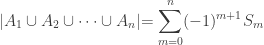
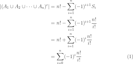
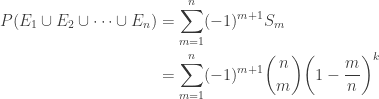
 ![\displaystyle (1) \ \ \ \ \ \ P[E_1 \cup E_2 \cup \cdots \cup E_n]=1-\frac{1}{2!}+\frac{1}{3!}-\cdots+(-1)^{n+1} \frac{1}{n!}](https://s0.wp.com/latex.php?latex=%5Cdisplaystyle+%281%29+%5C+%5C+%5C+%5C+%5C+%5C+P%5BE_1+%5Ccup+E_2+%5Ccup+%5Ccdots+%5Ccup+E_n%5D%3D1-%5Cfrac%7B1%7D%7B2%21%7D%2B%5Cfrac%7B1%7D%7B3%21%7D-%5Ccdots%2B%28-1%29%5E%7Bn%2B1%7D+%5Cfrac%7B1%7D%7Bn%21%7D&bg=ffffff&fg=333333&s=0&c=20201002)
 is obtained by using an idea called the inclusion-exclusion principle. We will get to that in just a minute. First let’s look at the results of
 ![\displaystyle (2) \ \ \ \ \ \ \begin{bmatrix} \text{n}&\text{ }& P[E_1 \cup E_2 \cup \cdots \cup E_n] \\\text{ }&\text{ }&\text{ } \\ 3&\text{ }&0.666667 \\ 4&\text{ }&0.625000 \\ 5&\text{ }&0.633333 \\ 6&\text{ }&0.631944 \\ 7&\text{ }&0.632143 \\ 8&\text{ }&0.632118 \\ 9&\text{ }&0.632121 \\ 10&\text{ }&0.632121 \\ 11&\text{ }&0.632121 \\ 12&\text{ }&0.632121 \end{bmatrix}](https://s0.wp.com/latex.php?latex=%5Cdisplaystyle+%282%29+%5C+%5C+%5C+%5C+%5C+%5C++%5Cbegin%7Bbmatrix%7D+%5Ctext%7Bn%7D%26%5Ctext%7B+%7D%26+P%5BE_1+%5Ccup+E_2+%5Ccup+%5Ccdots+%5Ccup+E_n%5D++%5C%5C%5Ctext%7B+%7D%26%5Ctext%7B+%7D%26%5Ctext%7B+%7D+%5C%5C+3%26%5Ctext%7B+%7D%260.666667++%5C%5C+4%26%5Ctext%7B+%7D%260.625000++%5C%5C+5%26%5Ctext%7B+%7D%260.633333++%5C%5C+6%26%5Ctext%7B+%7D%260.631944++%5C%5C+7%26%5Ctext%7B+%7D%260.632143++%5C%5C+8%26%5Ctext%7B+%7D%260.632118+%5C%5C+9%26%5Ctext%7B+%7D%260.632121+%5C%5C+10%26%5Ctext%7B+%7D%260.632121+%5C%5C+11%26%5Ctext%7B+%7D%260.632121+%5C%5C+12%26%5Ctext%7B+%7D%260.632121+%5Cend%7Bbmatrix%7D&bg=ffffff&fg=333333&s=-1&c=20201002)
 . We show that the probability in
 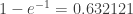 . Note that the Taylor’s series expansion of
 is:
is: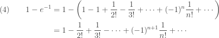
 is the probability in
 ![P[E_1 \cup E_2 \cup \cdots \cup E_n]](https://s0.wp.com/latex.php?latex=P%5BE_1+%5Ccup+E_2+%5Ccup+%5Ccdots+%5Ccup+E_n%5D&bg=ffffff&fg=333333&s=0&c=20201002) will be closer and closer to
will be closer and closer to  . We have:
![\displaystyle (5) \ \ \ \ \ \ \lim \limits_{n \rightarrow \infty} P[E_1 \cup E_2 \cup \cdots \cup E_n]=1 - e^{-1}](https://s0.wp.com/latex.php?latex=%5Cdisplaystyle+%285%29+%5C+%5C+%5C+%5C+%5C+%5C+%5Clim+%5Climits_%7Bn+%5Crightarrow+%5Cinfty%7D+P%5BE_1+%5Ccup+E_2+%5Ccup+%5Ccdots+%5Ccup+E_n%5D%3D1+-+e%5E%7B-1%7D&bg=ffffff&fg=333333&s=0&c=20201002)
![\displaystyle (6) \ \ \ \ \ \ \lim \limits_{n \rightarrow \infty} P[(E_1 \cup E_2 \cup \cdots \cup E_n)^c]=e^{-1}](https://s0.wp.com/latex.php?latex=%5Cdisplaystyle+%286%29+%5C+%5C+%5C+%5C+%5C+%5C+%5Clim+%5Climits_%7Bn+%5Crightarrow+%5Cinfty%7D+P%5B%28E_1+%5Ccup+E_2+%5Ccup+%5Ccdots+%5Ccup+E_n%29%5Ec%5D%3De%5E%7B-1%7D&bg=ffffff&fg=333333&s=0&c=20201002)
 says that it does not matter how many people are in the random gift exchange, the answer to the matching problem is always
  says that the probability of having no matches approaches
  to be more precise) that there is at least one match. So in a random gift exchange as described at the beginning, it is much easier to see a match than not to see one.
![\displaystyle (7) \ \ \ \ \ \ P[E_1 \cup E_2]=P[E_1]+P[E_1]-P[E_1 \cap E_2]](https://s0.wp.com/latex.php?latex=%5Cdisplaystyle+%287%29+%5C+%5C+%5C+%5C+%5C+%5C+P%5BE_1+%5Ccup+E_2%5D%3DP%5BE_1%5D%2BP%5BE_1%5D-P%5BE_1+%5Ccap+E_2%5D&bg=ffffff&fg=333333&s=0&c=20201002)
![\displaystyle \begin{aligned} (8) \ \ \ \ \ \ P[E_1 \cup E_2 \cup E_3]&=P[E_1]+P[E_1]+P[E_3] \\& \ \ \ \ -P[E_1 \cap E_2]-P[E_1 \cap E_3]-P[E_2 \cap E_3] \\& \ \ \ \ +P[E_1 \cap E_2 \cap E_3] \end{aligned}](https://s0.wp.com/latex.php?latex=%5Cdisplaystyle+%5Cbegin%7Baligned%7D+%288%29+%5C+%5C+%5C+%5C+%5C+%5C+++P%5BE_1+%5Ccup+E_2+%5Ccup+E_3%5D%26%3DP%5BE_1%5D%2BP%5BE_1%5D%2BP%5BE_3%5D+%5C%5C%26+%5C+%5C+%5C+%5C+-P%5BE_1+%5Ccap+E_2%5D-P%5BE_1+%5Ccap+E_3%5D-P%5BE_2+%5Ccap+E_3%5D+%5C%5C%26+%5C+%5C+%5C+%5C+%2BP%5BE_1+%5Ccap+E_2+%5Ccap+E_3%5D++%5Cend%7Baligned%7D&bg=ffffff&fg=333333&s=0&c=20201002)
 . Because the subtractions remove too much, we need to add back the probabilities of the intersections of three individual events
  . The process of inclusion and exclusion continues until we reach the step of adding/removing of the intersection
  . The following is the statement of the inclusion-exclusion principle.
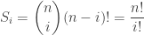
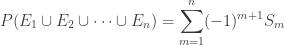
![\displaystyle (9) \ \ \ \ \ \ P[E_1 \cup E_2 \cdots \cup E_n]=S_1-S_2+S_3- \ \ \cdots \ \ +(-1)^{n+1}S_n](https://s0.wp.com/latex.php?latex=%5Cdisplaystyle+%289%29+%5C+%5C+%5C+%5C+%5C+%5C+P%5BE_1+%5Ccup+E_2+%5Ccdots+%5Ccup+E_n%5D%3DS_1-S_2%2BS_3-+%5C+%5C+%5Ccdots+%5C+%5C+%2B%28-1%29%5E%7Bn%2B1%7DS_n&bg=ffffff&fg=333333&s=0&c=20201002)
 ,
,  is the sum of all probabilities
 ![P[E_i]](https://s0.wp.com/latex.php?latex=P%5BE_i%5D&bg=ffffff&fg=333333&s=0&c=20201002) ,
,  is the sum of all possible probabilities of the intersection of two events
  and
and  is the sum of all possible probabilities of the intersection of three events and so on.
 people are free to select gifts. The probability of this event is
 ![\displaystyle P[E_i]=\frac{(n-1)!}{n!}](https://s0.wp.com/latex.php?latex=%5Cdisplaystyle+P%5BE_i%5D%3D%5Cfrac%7B%28n-1%29%21%7D%7Bn%21%7D&bg=ffffff&fg=333333&s=0&c=20201002) . There are
. There are 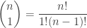 many ways of fixing 1 gift. So
 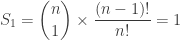 .
. person get their own gifts while the other
  people are free to select gifts. The probability of this event is
 ![\displaystyle P[E_i \cap E_j]=\frac{(n-2)!}{n!}](https://s0.wp.com/latex.php?latex=%5Cdisplaystyle+P%5BE_i+%5Ccap+E_j%5D%3D%5Cfrac%7B%28n-2%29%21%7D%7Bn%21%7D&bg=ffffff&fg=333333&s=0&c=20201002) . There are
. There are  many ways of fixing 2 gifts. So
  .
. and
and  and so on. Then plugging
  into
into  through
  is the
  ? On average, how many matches will there be? The number of matches is a random variable. We comment on this random variable resulting from the matching problem. We also derive the probability density function and its moments. We also comment the relation this random variable with the Poisson distribution.
 . The matching problem corresponds to the random selection of all the points in
  without replacement. The random selection of points of the entire set
  where each
  and
and  for
for  . These ordered samples are precisely the permutations of the set
  is selected in the
  ). The matching problem is a counting problem. We demonstrate how to count the
  :
:
 . The random variable
  , the following is the cardinality of the event
  :
: where the counts
  are defined by the following:


 , we have the familiar formula:
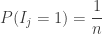
 be the event that the
  is the event that there is at least one match in the deck of
 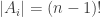 . As a result,
  .
. , the
, the  cards are free to permute. Thus we have
  and
and 

 of them have no matches. Thus the probability of having no matches in a shuffled deck of
 , we consider the event that
 . It is impossible to have exactly
  . There is only one permutation out of
  ,
, 
 and the Poisson desnity function with parameter
  . The following matrix shows the results (rounded to eight decimal places).
 converges to the Poisson distribution with parameter
  above converges to
  , which is the Poisson distribution with parameter
  above is the Taylor expansion of
  and the probability of at least one match is approximately
  . As the above example shows, the convergence occurs fairly rapidly.
 and
and  regardless of
  ,
,  is an indicator variable:
 and for all
  ,
,  . To see this, the event
  is the event
  defined in the derivation of the probability density function of
  . Thus the probability that the
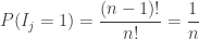
 is the event
  . Thus the probability that both the

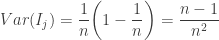
 , we need to find the covariance
  . Note that the indicator variables
 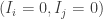 ,
,  ,
, 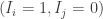 ,
,  . The only relevant case is the last one. Thus we have:
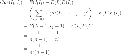

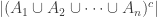
 cards, five fair dice are rolled. The resulting five scores from the dice form a poker dice hand. The possible hands are ranked as follows:
 ).
). ).
). ).
). ).
). ).
). ).
). ).
). dice, there are
  ordered outcomes. For example, assuming that the five dice are rolled one at a time,
  indicates outcome that the first die results in a two and the second die results in a three and so on (this is a three of a kind). To find the probability of a three of a kind, we simply divide the number of ways such hands can occur by
  . We use the multinomial coefficients to obtain the number of outcomes for each type of poker dice hands.
  cells. As will be shown below, the problem of computing the probabilities of poker dice hands is seen through the lens of the occupancy problem of randonly placing
  denotes a three of a kind hand of
  is also a three of a kind hand, representing the outcome that the score of one appearing three times, the score of two appearing one time and the score of three appearing one time. We use the multinomial coefficients to determine how many of the
 , four
  , four
  and two
  , there are
  possible
  -letter strings that can be formed, of which
  is one specific example.
 .
. two times, a
  one time, a
  . We are trying to partition
 possible hands,
  of them satisfiy the condition that a
 are examples of one pair. In essense, we need to count all the occupancy number sets such that among the
  and three of the cells are
  and one with two
  . The following is the multinomial coefficient (the second application of the multinomial theorem):
 and for a random poker dice hand, the probability that it is a one pair is:


 (Revised March 28, 2015)
 . Suppose we sample
 many ordered samples. Each character drawn has
  many ordered samples of size
  ,
,  ,
,  and
and  . We represent the unordered sample in two ways:

 , the number of
  many unordered samples. In general, if the population size is
  many unordered samples, either represented as
  calculated above. This is also the total number of non-negative integer solutions to the equation
  . Thinking of an unordered sample as a
  . Suppose that each letter is already selected once. Then we need to sample
  more times out of these
  . To generalize, if the population size is
  many unordered samples in which all objects in the population are represented in each sample.
 positions and so on.
 where
where  , the total number of ordered samples equivalent to this unordered sample is
  . As we shall see, these are called multinomial coefficients.
 many). We then collapse these ordered samples to just
  are non-negative integers:
 , which is the number of non-negative integer solutions to the equation
  . Each term
  in the polynomial expansion can be considered as an unordered sample in the finite sampling with replacement. Then the coefficient of each term (called multinomial coefficient) is the number of associated ordered samples. As a result, the multinomial coefficients sum to
 ) and we have
  many
many  ,
,  many
many  and so on, then the multinomial coefficient in
  . We have
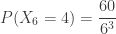
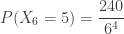
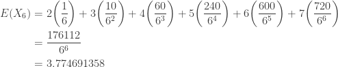
 . For a small restaurant with a daily customer count under three to four hundred, free dessert may not have to be offered at all. We will also show that the median number of customers until the arrival of the first birthday customer is
  . So if the daily customer count is less than
  % chance that a free dessert will not have to be offered. To obtain these results, we ignore leap year and assume that any day of the year is equally likely to be the birthday of a random customer. The results in this post will not hold if the free dessert offer is widely known and many customers come to the restaurant for the purpose of taking advantage of the free dessert offer.
 . Success here means a ball reaches the cell specified in advance. Let
  be the number of trials (placements of balls) until the first success. Then
  be any integer greater than
  be the number of trials until the


 is the same as the probability that there are no successes in the first

 . Let
. Let 


 success takes place after
  successes in the first
  . Note that


 (the probability that today is his or her birthday). Thus the mean number of customers until we see a birthday customer is

 . The median is
  .
.

 customers have arrived and there is no birthday customer. Would this mean that it is more likely that there will be a birthday customer in the next
  . Of course, we will discuss the connection with the birthday problem.
 and
and  .
. .
.
 , the probability of having different birthdays is
  . Thus there is more than
  people (
 ). On the other hand,
  and
and  . Thus among
  people, the probability of having a common birthday is less than
  .
. step. This means that the first
 . Then there are
 . This is the probability that it takes more than
  should agree with the probability stated in
 and
and
 .
. .
.


 .
.
 . Define
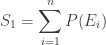


 or
or  , we have the following familiar formulas:

 be the number of empty cells. Then the probability that all cells are occupied (zero cell is empty) and the probability that exactly
 .
. . We proceed to derive the sums
  ways. Thus
  .
. ways. Thus we have
  .
.  , and so on. For
  , we have
 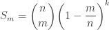 .
.

 cells and these remaining
 balls and
  cells. The probability of having
  empty cells. As in Theorem 2,
  is the number of empty cells when placing
  .
.