Hazard rate function | A Blog on Probability and Statistics

In this post, we introduce the hazard rate function using the notions of non-homogeneous Poisson process.

In a Poisson process, changes occur at a constant rate $\lambda$ per unit time. Suppose that we interpret the changes in a Poisson process from a mortality point of view, i.e. a change in the Poisson process mean a termination of a system, be it biological or manufactured, and this Poisson process counts the number of terminations as they occur. Then the rate of change $\lambda$ is interpreted as a hazard rate (or failure rate or force of mortality). With a constant force of mortality, the time until the next change is exponentially distributed. In this post, we discuss the hazard rate function in a more general setting. The process that counts of the number of terminations will no longer have a constant hazard rate, and instead will have a hazard rate function $\lambda(t)$ , a function of time $t$ . Such a counting process is called a non-homogeneous Poisson process. We discuss the survival probability models (the time to the first termination) associated with a non-homogeneous Poisson process. We then discuss several important examples of survival probability models, including the Weibull distribution, the Gompertz distribution and the model based on the Makeham’s law. See [1] for more information about the hazard rate function.

$\text{ }$

The Poisson Process
We start with the three postulates of a Poisson process. Consider an experiment in which the occurrences of a certain type of events are counted during a given time interval. We call the occurrence of the type of events in question a change. We assume the following three conditions:

The numbers of changes occurring in nonoverlapping intervals are independent.
The probability of two or more changes taking place in a sufficiently small interval is essentially zero.
The probability of exactly one change in the short interval $(t,t+\delta)$ is approximately $\lambda \delta$ where $\delta$ is sufficiently small and $\lambda$ is a positive constant.

$\text{ }$

When we interpret the Poisson process in a mortality point of view, the constant $\lambda$ is a hazard rate (or force of mortality), which can be interpreted as the rate of failure at the next instant given that the life has survived to time $t$ . With a constant force of mortality, the survival model (the time until the next termination) has an exponential distribution with mean $\frac{1}{\lambda}$ . We wish to relax the constant force of mortality assumption by making $\lambda$ a function of $t$ instead. The remainder of this post is based on the non-homogeneous Poisson process defined below.

$\text{ }$

The Non-Homogeneous Poisson Process
We modifiy condition 3 above by making $\lambda(t)$ a function of $t$ . We have the following modified counting process.

The numbers of changes occurring in nonoverlapping intervals are independent.
The probability of two or more changes taking place in a sufficiently small interval is essentially zero.
The probability of exactly one change in the short interval $(t,t+\delta)$ is approximately $\lambda(t) \delta$ where $\delta$ is sufficiently small and $\lambda(t)$ is a nonnegative function of $t$ .

$\text{ }$

We focus on the survival model aspect of such counting processes. Such process can be interpreted as models for the number of changes occurred in a time interval where a change means “termination” or ‘failure” of a system under consideration. The rate of change function $\lambda(t)$ indicated in condition 3 is called the hazard rate function. It is also called the failure rate function in reliability engineering and the force of mortality in life contingency theory.

Based on condition 3 in the non-homogeneous Poisson process, the hazard rate function $\lambda(t)$ can be interpreted as the rate of failure at the next instant given that the life has survived to time $t$ .

Two random variables naturally arise from a non-homogeneous Poisson process are described here. One is the discrete variable $N_t$ , defined as the number of changes in the time interval $(0,t)$ . The other is the continuous random variable $T$ , defined as the time until the occurrence of the first change. The probability distribution of $T$ is called a survival model. The following is the link between $N_t$ and $T$ .

$\text{ }$

$\displaystyle \begin{aligned}(1) \ \ \ \ \ \ \ \ \ &P[T > t]=P[N_t=0] \end{aligned}$

$\text{ }$

Note that $P[T > t]$ is the probability that the next change occurs after time $t$ . This means that there is no change within the interval $(0,t)$ . We have the following theorems.

$\text{ }$

Theorem 1.
Let 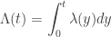$\displaystyle \Lambda(t)=\int_{0}^{t} \lambda(y) dy$ . Then $e^{-\Lambda(t)}$ is the probability that there is no change in the interval $(0,t)$ . That is, $\displaystyle P[N_t=0]=e^{-\Lambda(t)}$ .

Proof. We are interested in finding the probability of zero changes in the interval $(0,y+\delta)$ . By condition 1, the numbers of changes in the nonoverlapping intervals $(0,y)$ and $(y,y+\delta)$ are independent. Thus we have:

$\text{ }$

$\displaystyle (2) \ \ \ \ \ \ \ \ P[N_{y+\delta}=0] \approx P[N_y=0] \times [1-\lambda(y) \delta]$

$\text{ }$

Note that by condition 3, the probability of exactly one change in the small interval $(y,y+\delta)$ is $\lambda(y) \delta$ . Thus $[1-\lambda(y) \delta]$ is the probability of no change in the interval $(y,y+\delta)$ . Continuing with equation $(2)$ , we have the following derivation:

$\text{ }$

$\displaystyle \begin{aligned}. \ \ \ \ \ \ \ \ \ &\frac{P[N_{y+\delta}=0] - P[N_y=0]}{\delta} \approx -\lambda(y) P[N_y=0] \\&\text{ } \\&\frac{d}{dy} P[N_y=0]=-\lambda(y) P[N_y=0] \\&\text{ } \\&\frac{\frac{d}{dy} P[N_y=0]}{P[N_y=0]}=-\lambda(y) \\&\text{ } \\&\int_0^{t} \frac{\frac{d}{dy} P[N_y=0]}{P[N_y=0]} dy=-\int_0^{t} \lambda(y)dy \end{aligned}$

$\text{ }$

Evaluating the integral on the left hand side with the boundary condition of $P[N_0=0]=1$ produces the following results:

$\displaystyle \begin{aligned}. \ \ \ \ \ \ \ \ \ &ln P[N_t=0]=-\int_0^{t} \lambda(y)dy \\&\text{ } \\&P[N_t=0]=e^{\displaystyle -\int_0^{t} \lambda(y)dy} \end{aligned}$

$\text{ }$

Theorem 2
As discussed above, let $T$ be the length of the interval that is required to observe the first change. Then the following are the distribution function, survival function and pdf of $T$ :

$\displaystyle \begin{aligned}. \ \ \ \ \ \ \ \ \ &F_T(t)=\displaystyle 1-e^{\displaystyle -\int_0^t \lambda(y) dy} \\&\text{ } \\&S_T(t)=\displaystyle e^{\displaystyle -\int_0^t \lambda(y) dy} \\&\text{ } \\&f_T(t)=\displaystyle \lambda(t) \ e^{\displaystyle -\int_0^t \lambda(y) dy} \end{aligned}$

Proof. In Theorem 1, we derive the probability $P[N_y=0]$ for the discrete variable $N_y$ derived from the non-homogeneous Poisson process. We now consider the continuous random variable $T$ , the time until the first change, which is related to $N_t$ by $(1)$ . Thus $S_T(t)=P[T > t]=P[N_t=0]=e^{-\int_0^t \lambda(y) dy}$ . The distribution function and density function can be derived accordingly.

$\text{ }$

Theorem 3
The hazard rate function $\lambda(t)$ is equivalent to each of the following:

$\displaystyle \begin{aligned}. \ \ \ \ \ \ \ \ \ &\lambda(t)=\frac{f_T(t)}{1-F_T(t)} \\&\text{ } \\&\lambda(t)=\frac{-S_T^{'}(t)}{S_T(t)} \end{aligned}$

$\text{ }$

Remark
Theorem 1 and Theorem 2 show that in a non-homogeneous Poisson process as described above, the hazard rate function $\lambda(t)$ completely specifies the probability distribution of the survival model $T$ (the time until the first change) . Once the rate of change function $\lambda(t)$ is known in the non-homogeneous Poisson process, we can use it to generate the survival function $S_T(t)$ . All of the examples of survival models given below are derived by assuming the functional form of the hazard rate function. The result in Theorem 2 holds even outside the context of a non-homogeneous Poisson process, that is, given the hazard rate function $\lambda(t)$ , we can derive the three distributional items $S_T(t)$ , $F_T(t)$ , $f_T(t)$ .

The ratio in Theorem 3 indicates that the probability distribution determines the hazard rate function. In fact, the ratio in Theorem 3 is the usual definition of the hazard rate function. That is, the hazard rate function can be defined as the ratio of the density and the survival function (one minus the cdf). With this definition, we can also recover the survival function. Whenever $\displaystyle \lambda(x)=\frac{f_X(x)}{1-F_X(x)}$ , we can derive:

$\text{ }$

$\displaystyle \begin{aligned}. \ \ \ \ \ \ \ \ \ &S_X(x)=\displaystyle e^{-\int_0^t \lambda(y) dy} \end{aligned}$

$\text{ }$

As indicated above, the hazard rate function can be interpreted as the failure rate at time $t$ given that the life in question has survived to time $t$ . It is the rate of failure at the next instant given that the life or system being studied has survived up to time $t$ .

It is interesting to note that the function $\Lambda(t)=\int_0^t \lambda(y) dy$ defined in Theorem 1 is called the cumulative hazard rate function. Thus the cumulative hazard rate function is an alternative way of representing the hazard rate function (see the discussion on Weibull distribution below).

——————————————————————————————————————
Examples of Survival Models

–Exponential Distribution–
In many applications, especially those for biological organisms and mechanical systems that wear out over time, the hazard rate $\lambda(t)$ is an increasing function of $t$ . In other words, the older the life in question (the larger the $t$ ), the higher chance of failure at the next instant. For humans, the probability of a 85 years old dying in the next year is clearly higher than for a 20 years old. In a Poisson process, the rate of change $\lambda(t)=\lambda$ indicated in condition 3 is a constant. As a result, the time $T$ until the first change derived in Theorem 2 has an exponential distribution with parameter $\lambda$ . In terms of mortality study or reliability study of machines that wear out over time, this is not a realistic model. However, if the mortality or failure is caused by random external events, this could be an appropriate model.

–Weibull Distribution–
This distribution is an excellent model choice for describing the life of manufactured objects. It is defined by the following cumulative hazard rate function:

$\text{ }$

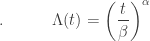$\displaystyle \begin{aligned}. \ \ \ \ \ \ \ \ \ &\Lambda(t)=\biggl(\frac{t}{\beta}\biggr)^{\alpha} \end{aligned}$ where $\alpha > 0$ and $\beta>0$

$\text{ }$

As a result, the hazard rate function, the density function and the survival function for the lifetime distribution are:

$\displaystyle \begin{aligned}. \ \ \ \ \ \ \ \ \ &\lambda(t)=\frac{\alpha}{\beta} \biggl(\frac{t}{\beta}\biggr)^{\alpha-1} \\&\text{ } \\&f_T(t)=\frac{\alpha}{\beta} \biggl(\frac{t}{\beta}\biggr)^{\alpha-1} \displaystyle e^{\displaystyle -\biggl[\frac{t}{\beta}\biggr]^{\alpha}} \\&\text{ } \\&S_T(t)=\displaystyle e^{\displaystyle -\biggl[\frac{t}{\beta}\biggr]^{\alpha}} \end{aligned}$

$\text{ }$

The parameter $\alpha$ is the shape parameter and $\beta$ is the scale parameter. When $\alpha=1$ , the hazard rate becomes a constant and the Weibull distribution becomes an exponential distribution.

When the parameter $\alpha<1$ , the failure rate decreases over time. One interpretation is that most of the defective items fail early on in the life cycle. Once they they are removed from the population, failure rate decreases over time.

When the parameter $1<\alpha$ , the failure rate increases with time. This is a good candidate for a model to describe the lifetime of machines or systems that wear out over time.

–The Gompertz Distribution–
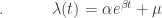
The Gompertz law states that the force of mortality or failure rate increases exponentially over time. It describe human mortality quite accurately. The following is the hazard rate function:

$\text{ }$

$\displaystyle \begin{aligned}. \ \ \ \ \ \ \ \ \ &\lambda(t)=\alpha e^{\beta t} \end{aligned}$ where $\alpha>0$ and $\beta>0$ .

$\text{ }$

The following are the cumulative hazard rate function as well as the survival function, distribution function and the pdf of the lifetime distribution $T$ .

$\text{ }$

$\displaystyle \begin{aligned}. \ \ \ \ \ \ \ \ \ &\Lambda(t)=\int_0^t \alpha e^{\beta y} dy=\frac{\alpha}{\beta} e^{\beta t}-\frac{\alpha}{\beta} \\&\text{ } \\&S_T(t)=\displaystyle e^{\displaystyle -\biggl(\frac{\alpha}{\beta} e^{\beta t}-\frac{\alpha}{\beta}\biggr)} \\&\text{ } \\&F_T(t)=\displaystyle 1-e^{\displaystyle -\biggl(\frac{\alpha}{\beta} e^{\beta t}-\frac{\alpha}{\beta}\biggr)} \\&\text{ } \\&f_T(t)=\displaystyle \alpha \ e^{\beta t} \ e^{\displaystyle -\biggl(\frac{\alpha}{\beta} e^{\beta t}-\frac{\alpha}{\beta}\biggr)} \end{aligned}$

$\text{ }$

–Makeham’s Law–
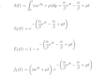
The Makeham’s Law states that the force of mortality is the Gompertz failure rate plus an age-indpendent component that accounts for external causes of mortality. The following is the hazard rate function:

$\text{ }$

$\displaystyle \begin{aligned}. \ \ \ \ \ \ \ \ \ &\lambda(t)=\alpha e^{\beta t}+\mu \end{aligned}$ where $\alpha>0$ , $\beta>0$ and $\mu>0$ .

$\text{ }$

The following are the cumulative hazard rate function as well as the survival function, distribution function and the pdf of the lifetime distribution $T$ .

$\text{ }$

$\displaystyle \begin{aligned}. \ \ \ \ \ \ \ \ \ &\Lambda(t)=\int_0^t (\alpha e^{\beta y}+\mu) dy=\frac{\alpha}{\beta} e^{\beta t}-\frac{\alpha}{\beta}+\mu t \\&\text{ } \\&S_T(t)=\displaystyle e^{\displaystyle -\biggl(\frac{\alpha}{\beta} e^{\beta t}-\frac{\alpha}{\beta}+\mu t\biggr)} \\&\text{ } \\&F_T(t)=\displaystyle 1-e^{\displaystyle -\biggl(\frac{\alpha}{\beta} e^{\beta t}-\frac{\alpha}{\beta}+\mu t\biggr)} \\&\text{ } \\&f_T(t)=\biggl( \alpha e^{\beta t}+\mu t \biggr) \ e^{\displaystyle -\biggl(\frac{\alpha}{\beta} e^{\beta t}-\frac{\alpha}{\beta}+\mu t\biggr)} \end{aligned}$

$\text{ }$

Reference

Klugman S.A., Panjer H. H., Wilmot G. E. Loss Models, From Data to Decisions, Second Edition., Wiley-Interscience, a John Wiley & Sons, Inc., New York, 2004